Keywords
|
| Differential equation; difference equation; homogeneous; linear; sequence; Oscillation and Non oscillation. |
INTRODUCTION
|
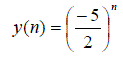
| Let us consider the nth term of sequence as an a(n) f (n) ? , for some unknown function f. For example, if |
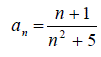 |
| then it is easy to compute explicitly, say, a0=1/5; a10=11/105; a100=101/10005. In such cases we are able to compute any given term in the sequence without reference to any other terms in the sequence. However it is often in the case of application that we do not begin with an explicit formula for the terms of a sequence; rather, we may know only some relationship between the various terms. An equation which expresses a value of a sequence as a function of the other terms in the sequence is called a difference equation. In particular, an equation which expresses the value an of a sequence ? ? an as a function of the term an?1 is called a first order difference equation. |
RELATED WORK
|
| In the recent years there has been a lot of interest in the study of oscillatory and non oscillatory properties of difference equations and functional difference equations. In the year 1966, S.N.Elaydi [ 4 ] was given some basic introduction about difference equations and briefly explained their oscillatory behaviors of solutions of difference equations. In the year 1999, R.P.Agarwal, and J.Popenda [ 2 ] were explained several new fundamental concepts in this fast developing area of research. These concepts are explained thorough examples and supported by simple results. In the year 2000, Dan Sloughter [ 3 ] was explained the applications of difference equations with some real time examples. |
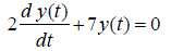
| Consider a homogeneous, first order, linear, differential equation of the form |
 (1) (1) |
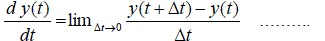
| in equation (1) t is the independent variable and y is the dependent variable , a function of t. We can do this by approximating derivatives by finite differences. Recall these definition of a derivative, |
 (2) (2) |
| at any point at which y(t) is differentiable. A derivative in continuous time can be approximated by finite differences in discrete time by |
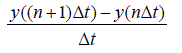 |
| This is called a forward difference because it uses the present or current value of y of y(nΔt) and the next or future value of y of y((n+1)Δt). Similarly |
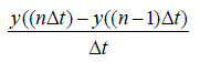 is a backward difference and is a backward difference and 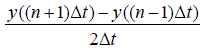 |
| is a central difference. In the limit as Δt approaches zero these are all the same, but in discrete time, Δt is fixed and is not zero and these three approximations to a continuous time derivative are , in general ,different. |
| As an illustration we will convert the differential equation (1) , into a difference equation by difference approximation, |
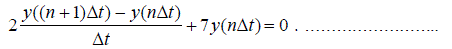 (3) (3) |
| To simplify the notation, let y[n] = y (nΔt) where the square brackets, [.], distinguish a function of discrete time from a function of continuous time which is indicated y using parenthesis, (.). In this notation, time is not explicitly indicated but, since the time between consecutive discrete-time values of the function, y is always Δt, we do not need to explicitly indicate time. Using the simplified notation, (3) becomes |
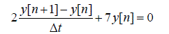 |
| 2(y [n+1] – y[n]) + 7Δty[n] =0 ………… |
| Which is a homogeneous difference equation. |
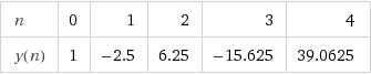
| The equation (4) is written as 7 y (n) + 2(y (n+1) – y (n)) = 0, with y (0) =1 |
| The solution of this equation is |
 And the graph of the equation is And the graph of the equation is |
 |
METHODOLOGY
|
Definition:
|
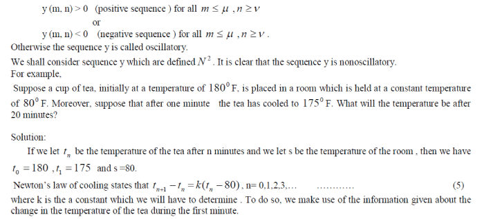
A sequence  is said to be nonoscillatory around 0 if there exist a positive integer ? such that is said to be nonoscillatory around 0 if there exist a positive integer ? such that |
 |
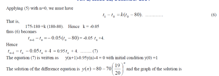 |
| for n= 0,1,2,3,… now (7) is in the standard form of a first order linear equation, so |
| let us take the first order linear difference equation is of the form |
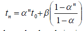 |
| we know that the solution is |
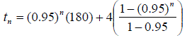 where α =0.95,β =4 and t0 =180 where α =0.95,β =4 and t0 =180 |
 ...... ...... |
| for n =0,1,2,3,… In particular, |
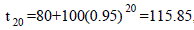 |
| where we have rounded the answer to two decimal places. Hence after 20 minutes the tea has cooled to just 116 0 F. Also, since |
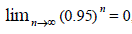 |
| we see that |
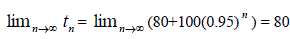 |
| that is , as we would expect, the temperature of the tea will approach an equilibrium temperature of 800 F, the room temperature . In figure 1 we have plotted temperature n t verses time n for n= 0,1,2,3,…,60, along with the horizontal line t = 80. As indicated by (10), we can see that n t decreases asymptotically towards 800 F as n increases. |
CONCLUSION
|
By the definition of nonoscillatory and based on some theorems, the solution of the given difference equation 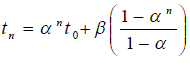 is nonoscillatory . is nonoscillatory . |
Figures at a glance
|
 |
 |
 |
| Figure 1 |
Figure 2 |
Figure 3 |
|
| |
References
|
- R.P.Agarwal,”Difference Equations and Inequalities”, Marcel Dekker, New York, 2000.
- R.P.Agarwal, and J.Popenda .” On the Oscillations of Recurrence Equations”, Nonlinear Analysis Vol.36, pp. 231-268, 1999.
- Dan Sloughter , “Difference equations “(section 1.4) , 2000.
- S.N.Elaydi.” An Introduction To Difference Equations”. Springer- Verlag, New York, 1996.
- H.A.El-Morshedy and S.R.Grace ,” Oscillation of Some Nonlinear Difference Equations.” J.Math.Anal.Appl.Vol.281, pp10-21, 2003.
- P.Mohankumar,A.Balasubramanian and A.Ramesh.,” Oscillatory Results of third Order Nonlinear Mixed Type Difference Equations.”,International Journal of Mathematical Archive-Vol.5(8),pp. 191-197,2014.
- Zdzislaw Sz afranski, Blazej szmanda.,“Oscillation of Solution of Some non-Linear Difference Equations”, Publications Mathematiques, Vol.40,pp.127-133,1996.
|