International Journal of Innovative Research in Science, Engineering and Technology
ISSN ONLINE(2319-8753)PRINT(2347-6710)
ISSN ONLINE(2319-8753)PRINT(2347-6710)
Yuvaraj S.A.1 Selvakumnar2
|
| Related article at Pubmed, Scholar Google |
Visit for more related articles at International Journal of Innovative Research in Science, Engineering and Technology
Target finding without predicted information of the target is one of the critical areas of development, the major area here propose a new sensor selection solution that improves the accuracy of target localization without prior knowledge of the target in wireless visual sensor networks. The proposed solution exploits the properties of the overlap region of the target in images: the more overlap grade, the more cameras project images of the target in the same direction; the greater overlap area, the higher possibility that the target is located in the region. The authors formulate the sensor selection problem as one of maximising the utility of multiplying the overlap grade by the overlap area gained from a set of sensors. Simulation results show the effectiveness of this approach of sensor selection in terms of improving the accuracy of target localization.
INTRODUCTION |
| Wireless visual sensor network (WVSN) is a particular type of wireless sensor network, which includes some nodes that are equipped with visual sensors. These visual sensors have a unique feature so that the targets covered by the camera can be far away from the sensor nodes, which enable WVSN to be adept in various security and surveillance applications, such as remote and distributed video-based surveillance, ambient assisted living and personal care etc [1]. For most applications of surveillance and monitoring, users are interested not only in the existence of some targets but also in the locations of these targets [2]. Therefore localisation is an extremely crucial service in WVSN, which contains self-localisations of sensor nodes and target localisation. In this paper, we mainly focus on the problem of target localisation. |
| Most of the previous research on target localisation in wireless scalar sensor networks has focused on acoustic and RF-based measurements as a means to determine fine- grained localization These measurement techniques can be broadly classified into three categories: angle of arrival (AOA) measurements, distance-related easurements and RSS profiling techniques [3]. However, these existing localisation algorithms cannot solve the target localization issue in WVSNs [4], because of the significant differences in information acquiring and processing methods from conventional sensor networks. Actually, vision-based target localisation in visual sensor networks will face great challenges. First, camera sensors generate a huge amount of data compared with scalar sensors, but such data processing is in general computationally expensive and is costly to implement locally. Besides, information on the depth dimension of the target is lost in the images. To ascertain depth, another camera is needed. Thus, target localization using multiple cameras has attracted much attention. The accuracy of the target localisation can be gradually improved by selecting the most informative cameras. However, since the delivery of visual information needs very high bandwidth, it is very difficult to transmit all the raw data from the sensors to the base station. Moreover, in WVSN, the visual sensor node is usually equipped with a low- resolution camera because of the cost limitation [5], which would probably incur some image distortion or ambiguity. If this kind of image is used to determine the target’s position, the accuracy will deteriorate. Furthermore, there might be partial occlusions in the interested area because of static objects such as partitions, tables etc. If a camera cannot see a considerable portion of the target, it should be discarded from the feasible set of cameras [6]. The reason behind this is that it contains too little position information, and it will be harmful for the accuracy of target localisation. Therefore it is necessary to select the set of camera nodes that can provide the most accurate position information of the target. Unfortunately, the problem of selecting the optimal set of camera sensors to participate in the target localisation process has not been fully addressed in the literatures. |
| In this paper, we mainly focus on camera sensors selection for locating a target in WVSN. Our purpose is to select the set of camera sensors for improving the accuracy of target localisation without any prior knowledge about the target. We introduce a typical epipolar geometrical model for computing target position. Then, we develop a novel criterion of camera sensors selection. The relationships between the overlap grade and the area of the overlap region of target in the images being taken from different cameras are analysed in this paper. On the basis of the properties of the overlap region, we develop a utility function for finding the optimal set of cameras involved in the target localisation. Thus, in order to find a subset of camera sensors that could produce the maximal utility, we map the camera sensor selection into an optimization problem. To evaluate the performance of the proposed sensor selection strategy in the improvement of target localisation accuracy, we make some comparisons with other node selection methods via some simulations. |
| Our main contributions include the following: (i) we design the overlap grade and the overlap area of the region of the target in images to describe the overlap extent of the target observed by cameras; (ii) based on the overlap grade and overlap area, an optimal camera selection algorithm is proposed with the goal of improving the accuracy of target localisation without any prior information of the target. The remainder of this paper is organised as follows. In Section 2, we briefly highlight the related works. Section 3 presents the epipolar geometrical model to compute the possible position of target. Section 4 defines the criterion and the utility function of sensor selection. Section 5 conducts experiments to validate and evaluate our proposed scheme and conclusions are given in Section 6. |
2 RELATED WORKS |
| Recently, research on image sensor networks has received some interest. However, only limited studies of the target localisation problem have been reported for WVSN. Farrell et al. [7] used a set of two cameras to locate the sensor nodes in WVSN. Unfortunately, they estimated the location of a target using non-imaging sensors. Massey et al. [8] proposed methods to implement localisation using camera networks. They discussed the grid-based coordination scheme and the convex polygon intersection scheme for determining a target’s position in the global coordinate space. Oztarak et al. [9] used the distance from the camera to the extracted target to obtain the relative accurate target localisation. Besides, some researchers used scaleinvariant feature transform (SIFT) to find feature point correlations for computing the coordinate of the target [10]. SIFT is an opportunistic feature point detection and correlation algorithm, but it has high processing and communication costs. Medeiros et al. [11] and Kurillo et al. [12] waved a bar with an LED light at each end to provide correlated feature points by the solutions that use the known length of the bar to fix the units of relative camera positions. |
| The problems related with the selection of cameras in WVSN have also been previously investigated. Camera selection is undertaken with the goal that the visual information from selected cameras should satisfy the specific application requirements. Thus, camera selection policies are directed by the applications. Different requirements of applications would lead to dramatically different criterions and methodologies of camera selection. In [13], the authors described a camera network node subset selection methodology for target localisation in the presence of static and moving occluders, which is based on the assumption that the object position is Gaussian random vector. Liu et al. [2] have designed cost and utility functions to map the sensor node selection problem into an optimisation problem and then proposed an optimal node- selection algorithm to select a subset of camera sensor for estimating the location of a target. Wang et al. [14] have proposed an entropy-based algorithm for selecting sensor nodes. It is also assumed that measurement of uncertainty of the target position approximated by the Gaussian distribution. In [15], the authors presented a method that selected cameras that minimised, the difference between the images provided by the selected cameras and the image captured by a real camera from the desired viewpoint. |
| Another sensor selection method based on the mutual information principle was presented in [16]. Recently, an entropy-based heuristic approach was proposed [17] which rapidly selected the next sensor to reduce overall uncertainty. In these approaches, the performance of the sensor selection algorithm was verified experimentally. These approaches were shown to be equivalent to minimising the expected posterior uncertainty. Dai and Akyildiz [18] have developed a correlation-based camera selection algorithm based on the proposed correlation function and entropy-based analytical framework. |
| From aforementioned works, we can observe that all these methods need some prior information about target, such as the probability distribution of the target location, the posterior probability density function of the target position, the image of the desired viewpoint etc., which cannot be accepted in practice. Without the prior information of the target, it would necessarily result in decreasing the accuracy of positioning, by their approaches. To overcome this problem, we analyse the properties of the overlap region of the target observed by cameras with overlapped field of views (FOV), and present a new camera sensor selection scheme without prior information of target. |
3 GENERAL TARGET LOCALISATION MODEL |
| We assume that the cameras are placed horizontally around a room, which is the most relevant case for many real world applications. We set up a world coordinate system oxwywzw for the area of interest. The xwoyw plane is the ground plane. We assume that each camera node in the network is aware of its own location in the world coordinate plane xwoyw. Also, each camera node in the network is aware of its orientation against a global axis in the coordinate plane. The xocy plane is set as the image plane of cameras. For a camera sensor, its optical centre can be denoted as oc. |
| Cameras project a target from a three-dimensional (3D) world to a 2D plane via a perspective point. Since a single camera node can only acquire the bearing of the target in visual image, localisation can only be achieved by fusing the information from multiple camera sensors. Thus, being distinct from traditional scalar sensors, the sensing capability of a camera is characterised by directional sensing. |
| The principle of computing the target’s position is to estimate the bearing of the target in each image. The bearings in the images of two different cameras can be intersected in a unique area that is the possible target position area. Specifically, as shown in Fig. 1, a camera has a FOV that represents the area on the xwoyw plane where a target captured by the camera is located. The FOV is represented as an isosceles triangle, where both the equal sides join at a point representing the camera location. The angle between these equal sides is known as the FOV angle and is a factory specification defined for every camera. We can limit the location of the target into a subarea in the FOV. In [8], they call this sub-area the location area of the camera. Location areas of different cameras that have intersections could generate a common sub-region, which is called the overlap region of the target where the target is probably located. |
 |
| The edge of the overlap region can be determined via the intersection area of the location of the cameras. The coordinates of the intersection points in the world coordinate plane can be calculated as follows. The target is represented as pixels on the image plane by a perspective projection model, as shown in Fig. 2. px1 and px2 are the observation measurements of the target’s border points in horizontal on the image coordinate system. On the basis of the pixel information, we can compute the bearing of the target in the world coordinate frame. The bearings of one of the target’s edges in the image of the camera can be computed according to the following formula |
| k = tan(w- arctan((2px/p) tan(u/2))) |
| Where k is the orientation of the target, w is the angel of camera, rotating around zw-axis, when the direction of the camera is along with the xw, w ¼ 0 and rotating in counter-clockwise is positive; u is the horizontal FOV and p is the number of pixels in horizontal. px is the horizontal pixel coordinate in the image. In our localisation scheme, only px is communicated to the central unit. If two cameras capture the same target at the same time, the target’s bearings generated from two cameras could be intersected. We can infer the coordinates of the intersected points of bearings from the known positions of two cameras. The computation process is described by the following equation |
 |
| where ki is the bearing of the target in ith camera’s image; xci, yci are the coordinates of the ith camera in the world coordinate frame; x and y are the pending coordinates of the target in the world coordinate frame. The values x and y cannot be uniquely determined by a single camera. Thus, at least two cameras that detect the target are needed to determine the target’s position. The target position’s computation matrices are shown as follows |
 |
 |
| The coordinates of all the intersection points can be calculated by the above procedure. When all the intersection points are determined, the vertices of the overlap region are correspondingly decided. Therefore the overlap region of the target can be uniquely confirmed. |
4 Sensor selection strategies |
| Although only two cameras could determine an overlap region of the target, multiple cameras can add finer details about the location of the target by locating it in a smaller and smaller area. Generally, the accuracy of the target localisation can be gradually improved by selecting the most informative cameras till the required accuracy level of target state is achieved. However, image distortion/ ambiguity and object occlusion will undermine the accuracy of target localisation. Target position information that comes from certain cameras would include some errors. Accordingly, the accuracy of the final fusion result will deteriorate. It is inappropriate for all available camera sensors to participate in the localisation. In the practical application of localisation, therefore, in order to minimize the negative effects of errors from certain cameras, addressing the tradeoff between localisation quality and the number of measurements become very important. As a result, selecting a proper group of cameras from the available cameras set to perform target localisation is of research value. The major objective of our work is to properly determine the optimal set of cameras sensors for target localisation in a centralised way. Before going into detail, it is required to make some assumptions. Without loss of generality, we are given a set C ¼ {c1, c2, . . . , cn} of sensors with fixed lens in a 2D interested area; their locations and bearings are also given; one target is located in the views of cameras; and we assume that any information about the target is not previously known. |
4.1 Overlap grade of target region |
| If location areas of multiple cameras have intersected in a common region, this common region has multiple overlaps. Obviously, the common region with more overlaps reveals that more cameras locate the target in the same area. From the perspective of statistics, the region with more overlaps has the higher possibility that the target is located in the region. Therefore it is desirable to select cameras, which could generate the common region with the more overlaps to participate in the target localisation. |
| Overlap grade is the intersection times of the location areas of the target, whose concept is introduced to evaluate the overlap extent of the overlap region of the target. If the overlap region is generated by two cameras, the overlap grade of the region is 1, because the overlap region has been intersected only once. If the overlap region is generated by three different cameras, the overlap grade of the region is 3, because of the location area of the first camera intercrossing with that of the second and the third cameras; and the location area of the second camera is also intercrossed with that of the third camera in the same area, and the rest of the cameras in the location area can be arranged in the same manner. In fact, each intersection of location area of cameras contributes to 1 overlap grade. If an overlap region of target is composed of m cameras’ views, its overlap grade is the combination of any two different cameras from m cameras. The computing process of overlap grade could be formulised as follows |
| where Gm is the overlap grade. m is the number of nodes the set of cameras involved in merging the overlap region of the target. |
| From the perspective of the overlap grade, it is desirable to select the set of cameras, which could produce the maximum overlap grade. The greater overlap grade the overlap region of the target has, the more cameras that project the views of the target in the same location are in the global coordinate. The overlap region of the target, which has a greater overlap grade shows that the target is located in the region with the higher possibility in the global coordinate. However, the overlap grade could not reveal quantity and quality of the target’s position information. It is not enough to only rely on the overlap grade to determine the sensor set being involved in the target localisation. |
| 4.2 Overlap area of target region |
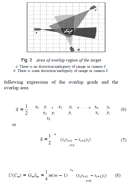
| From the perspective of image processing, the bigger target size of the image could provide more position information. Through the data fusion of multiple cameras the size of target can be expressed by area of the overlap region of the target. The area of overlap region of the target, which is called ‘overlap’ area in this study, reflects the affluent extent of the target’s location information. It will be illustrated by an example. As shown in Fig. 3, the parameters of all cameras and the position of target are exactly the same in two scenarios. If there is some distortion/ambiguity of image in the camera C in the second scenario, the overlap area fused by the three cameras is notably different between the two scenarios. The results of target localisation in the two scenarios are consequently different from each other. In the first scenario, shown as in Fig. 3a, the target is located in the centre of the pentagon shown as the black frame in the figure. In contrast, the position of the target in the second scenario will be in the centre of the triangle, as shown in Fig. 3b, which leads to some deflection from the real position of the target. Therefore the overlap area also dramatically affects the accuracy of overlap region of the target. |
| On the basis of the calculation procedure of intersection points described in Section 2, we can decide all the vertices of the overlap region of the target. This overlap region will always be a convex polygon [8]. Utilising the method of computing the union of two convex polygons, which is described in [19], we can distinguish the overlap region and order its vertices. Thus, according to the properties of the polygon, if the vertices are ordered counterclockwise, the area of the convex polygon can be computed by the |
 |
 |
| where S is the overlap area and n is the number of vertices of the polygon. (xi , yi) are the coordinates of the ith vertex of the overlap region of the target. Note that, to close the polygon, the first and the last vertex are the same, that is, (xn , yn) ¼ (x0, y0).Since the target’s size is shown as a sub-area in the image, the overlap area reveals the superposition of sub-areas by multiple cameras. In general, the greater overlap area can increase the likelihood of finding the region where the target is located. From this perspective, it is desirable to select the set of cameras that have to produce the maximum overlap area. |
4.3 Utility function f sensor-selection |
| In order to locate the target accurately, not only the greater overlap grade but also the larger overlap area should be needed by the overlap region of the target. The greater overlap grade requires that more cameras are involved in generating the overlap region. The larger overlap area requires bearings of the target in the images of cameras to project towards the same region as much as possible. Nevertheless, with the increase of cameras participating in the target localisation, the overlap area will certainly shirk. The comparison of the overlap area should be taken in the involvement of many cameras. Therefore we have to make a compromise between the area of the overlap region and the number of cameras that participate in forming the overlap region. |
| In order to obtain the more accurate location of the target, the preferable way is to select the camera group, which could generate the overlap region of target with maximal overlap grade and maximum overlap area. We could map the sensor selection problem (SSP) into an optimisation problem. |
| Therefore we present a utility function to find this set of camera sensors, as shown in (8), which returns the product where U is the utility function; Cm is a set of m cameras, m ≤ n; Gm and Sm are the overlap grade and the area of the overlap region of the target generated by the set of cameras Cm, respectively; vm is the vertices number of the overlap region of the target which is composed by the camera set Cm; and xi , yi are the coordinates of the ith vertex of the overlap region. |
| The optimal set has to generate the region of the target with the maximum product by multiplying the overlap grade by the overlap area. Therefore the SSP for improving the accuracy of target localisation is switched to the problem of finding the set of cameras with the maximal utility |
 |
| Its solution returns the optimal set of sensors formaximising utility. Our goal is to find the optimal set ofcameras Cm which could produce the maximum utility U from the C. |
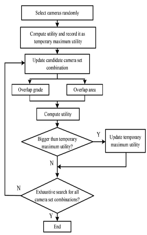
| The flow chart of sensor selection based on the proposed utility is illustrated as in Fig. 4. A camera set is randomly selected at the beginning. We introduce this set into (8) to compute the utility and record it as temporary maximum one. Then we update the candidate camera set and compute its utility. The utility is compared with the temporary maximum one. If it exceeds the maximum utility, the temporary maximum utility is updated. Otherwise, a judgement has to be made to check if all camera set combinations have been exhaustively searched. If so, the selection process will terminate, and the camera set, which produces the maximum utility is considered as the optimal camera set. If not, we have to go back to update the candidate camera set. Note that since methods of solving the set combination problem are not the main emphasis of our research, we should utilise the exhaustive search method |
| After sensor selection, we confirm the region where the target is located with higher possibility. In theory, the target could be located in any position in the region. We use the centroid of the overlap region to present coordinates of the target. According to the properties of the polygon, the centroid can be calculated by the following expression |
 |
| where Tx and Ty are the estimated coordinates of the target. |
4.4 Running time of the proposed sensorselection |
method |
| In this section, we analyse the time complexity of the proposed approach. As mentioned above, we know that the proposed approach is divided into overlap grade computation and overlap area computation. Overlap grade can be found in O(n) time. The running time of computing the overlap area mainly converges at the time of determining the overlap region. We utilised the algorithm described in [19] to compute the union of two polygons, which can be found in O(n1 + n2). n1 and n2 are the numbers of edges of two polygons respectively. In our case, because of the properties of camera sensors, any FOV of two sensors could be intersected at four points at most. |
| Accordingly, two cameras can only intersect in a quadrangle area. With the increase of cameras that are involved in the fusion of target localisation, the numbers of edges of the overlap region cannot exceed 2n. The overlap region can certainly be found in O(2n). Therefore the time complexity of our proposed sensor selection algorithm is O(n + 2n) �� O(2n). |
5 CASE STUDY AND SIMULATION RESULTS |
| We perform some simulation experiments to evaluate the performance of our proposed sensor selection algorithm in the accuracy improvement of the target localisation. The goal of the experiment is to locate a target in 2D plane in the world frame. |
5.1 Performance in accuracy improving of our roposed approach |
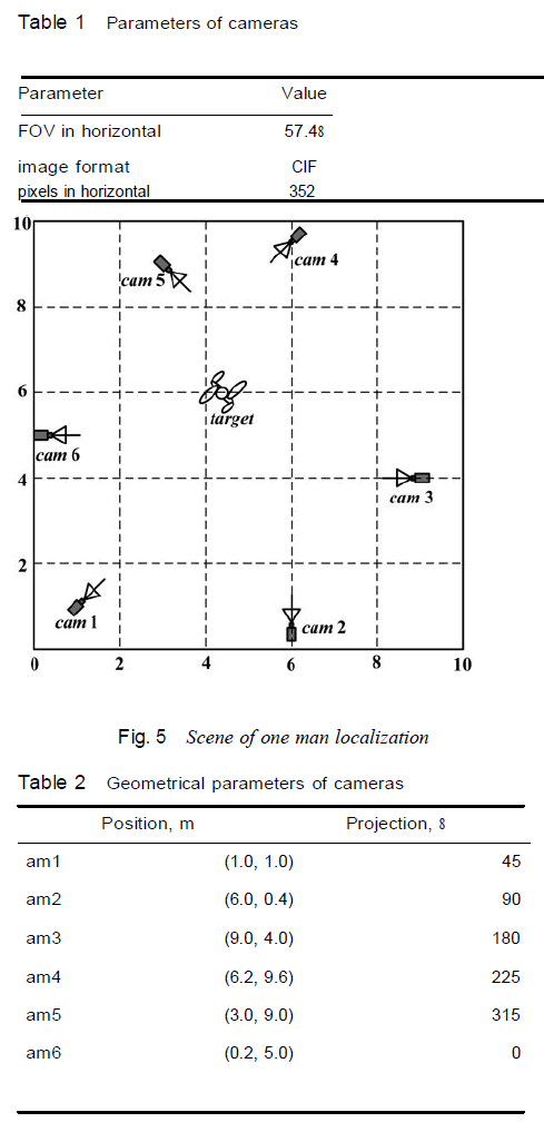
| For the reason of reducing the simulation complexity, we deployed six camera sensors in a 10 × 10 m field. The cameras are calibrated. The parameters of cameras are summarised in Table 1. Their locations and projection bearings with respect to a common world frame are shown in Fig. 5 and Table 2. A target is located at (4.40 and 6.00 m). The images taken from the six cameras are shown in Fig. 6. |
| We assume that the simple background subtraction is performed to extract the minimum boundary rectangle of the target. In this method, the background model updating is achieved in a pixel-based method, which periodically updates the background model to adapt to illumination changes. With the updated background model, a foreground region can easily be detected. A background subtraction method is effective for target extraction, particularly when the computation ability is low. |
 |
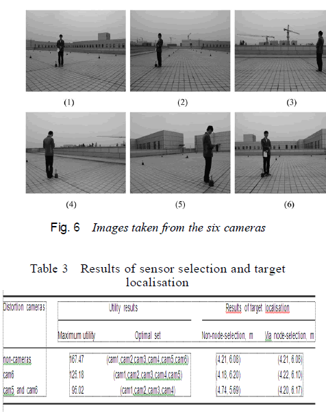 |
| In the first experiment, if there is no obvious istortion in images taken by the cameras, all the six cameras can be selected in the fusion of target localisation by our algorithm. The accuracy level is the same in both two approaches. In the second experiment, we artificially add some distortions on the image of the camera 6. According to our sensor selection algorithm, the other five cameras are selected in the target localisation, which could achieve the maximum utility. The error in the proposed approach is less than that in the non-node-selection approach. In the third experiment, we make the target’s images of camera 5 and camera 6 distorted. After sensor selection by our proposed algorithm, {cam1, cam2, cam3 and cam4} have been selected to be involved in target localisation. Both cam5 and cam6, with distortions in their images have been discarded from target localisation. The result of error of target localisation is about 0.26 m by our proposed approach. In contrast, the error is about 0.46 by the non- node-selection approach. This case indicates that our proposed method could select the optimal set of cameras for locating the target in the goal of improving the accuracy of target localisation. Besides, it also reveals that when some distortion or ambiguity occurs in certain cameras, it is not an appropriate way to include as many cameras as possible in the target localisation, due to accuracy deterioration incurred by distortion or ambiguity. |
5.2 Experimental evaluation of our proposed method |
| In this section, we perform simulations to evaluate the effectiveness of our proposed algorithm in the following assumption: the amount of sensors, which are involved in the target localisation is previously decided, but the specific cameras are not selected. |
| We take the blind near neighbourhood selection scheme as a reference, because most of camera selection methods cannot be used when there is no any prior information of the target. We compare our proposed method with the blind near neighbourhood selection schemes with the goal of improving the accuracy of target localisation. |
| 1. Blind near neighbourhood selection: randomly select the first camera, and then select the closest node from the remaining cameras till M cameras have been selected. Without loss of generality, for each M, repeat the experiment for ten times. Compute the target’s position at each time, and take the average value of the ten trials as the final position results. |
| 2. Our proposed method: the goal is to select M cameras from the N cameras to achieve the maximal utility. For each M, we could obtain a unique result of sensor selection. |
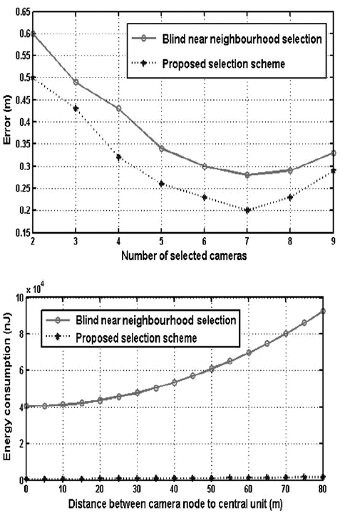
| In our experiment, we deploy ten cameras in the field (N ¼ 10). As mentioned in the foregoing, we assume that all the cameras are calibrated. In the precondition of knowing the locations and orientations of the cameras, all of the cameras can capture the target. We artificially add some distortions on three of the ten cameras. Let the number of cameras M selected for participating in the target localisation changes from 2 to 9. The errors of target localisation by the two schemes are shown in Fig. 7, where the real line and the spot line show the errors of target localisation in the blind near neighbourhood selection and in our proposed selection method, respectively. Fig. 7 plots the error performance of both schemes. The red real line and the blue spot line show the errors of target localisation in the blind near neighbourhood selection and in our proposed selection method, respectively. It is obvious that our proposed method has lower error level than the blind near neighbourhood selection when the same amount of sensors is selected. We find in both schemes that the errors of localisation decrease as the number of selected nodes increases when the selected sensors are less than 7. If the selected sensors are more than 7, the accuracy of target localisation begins to deteriorate. In this case, it is consistent with the fact that we have added some distortions on three of the ten cameras’ images. If we want to obtain the same accuracy of target localisation, the sensors that have to be selected by blind near neighbourhood selection are more than that in the proposed method. Therefore given the number of sensors need to be selected, our proposed method gets more accurate results than the blind near neighbourhood selection does. |
| It is commonly believed that communication is the most energy consuming operation in sensors, which requires much more energy than processing. According to the energy model for communications in [20], we can calculate the energy consumption for communication from camera nodes to the central unit. A comparison of energy consumption for communication is illustrated in Fig. 8. For both schemes, the energy consumption increases as the distance between the camera nodes to the central unit increases. However, the proposed selection method requires much less energy for communication than the blind near neighbourhood selection does. In our proposed method, the reason behind this is that only the positions of two pixels are required to transmit to the central unit. |
 |
6 CONCLUSIONS |
| We have presented a utility-based sensor selection solution by selecting the optimal set of cameras for improving the accuracy of target localization without prior knowledge of the target in the WVSNs. With the help of numerical simulations we show that the proposed solution can select the most informative cameras with little communication energy consumption. Therefore the proposed sensor selection scheme serves as a useful tool for selecting the sensors in improving the accuracy of target localisation. Also, independence of prior knowledge of the target makes our proposed method more suitable for non-collaborative applications. |
References |
|