International Journal of Innovative Research in Science, Engineering and Technology
ISSN ONLINE(2319-8753)PRINT(2347-6710)
ISSN ONLINE(2319-8753)PRINT(2347-6710)
Ravi.H.C1, Madhukeshwara.N2, S.Kumarappa3
|
| Related article at Pubmed, Scholar Google |
Visit for more related articles at International Journal of Innovative Research in Science, Engineering and Technology
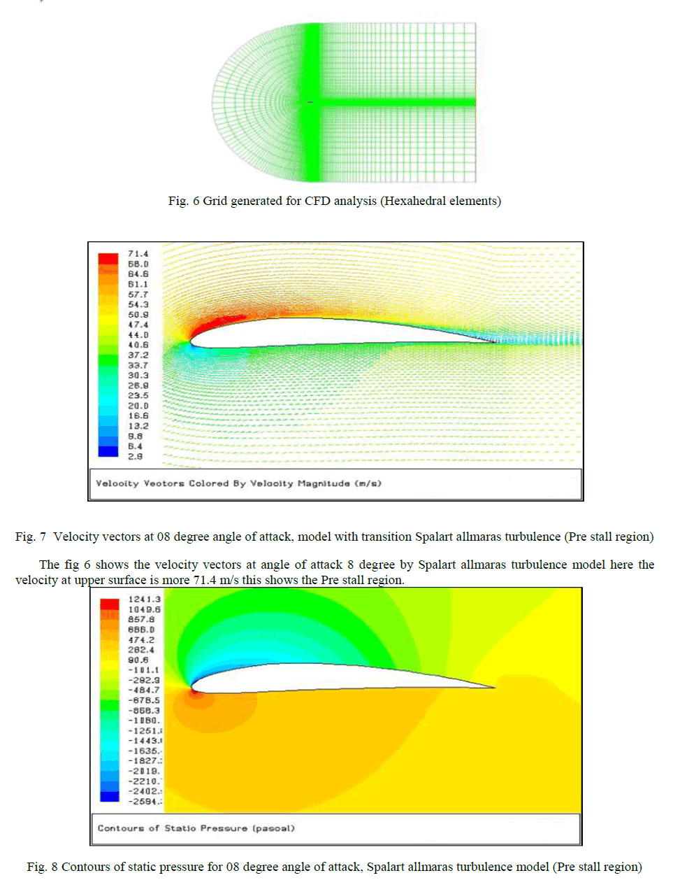
Numerical investigation of aerodynamics phenomena in the post stall region using Computational Fluid Dynamics is critical task due to the strong vortex dynamics involved. Literatures cited in this filed indicates that the Turbulence models employed in most of the commercial CFD software’s will assume the boundary layer around the airfoil as fully turbulent and hence the physical phenomena is wrongly addressed and also this approximation will lead to deviation in results from experimentally measured data in the post stall region. Research in this area concluded that the flow transition (boundary layer transition) from laminar to turbulent around the surface of the airfoil needs to be properly implemented in CFD analysis in order to have a reliable prediction in post stall region. This work aims in predicting the flow transition from laminar to turbulent for flow over NACA4412 airfoil in the incompressible flow regime.CFD analysis methodology involves the use of Mentors Shear Stress Transport Turbulence model(k-ω model)with transitional flow option.CFD analysis results are compared with wind tunnel test data.CFD analysis is also carried out with Spalart allmaras turbulence model which assumes the boundary layer as fully turbulent.
Keywords |
| CFD, Transition, SST model, Turbulence, Stall |
INTRODUCTION |
| The rapid evolution of computational fluid dynamics (CFD) has been driven by the need for faster and more accurate methods for the calculations of flow fields around configurations of technical interest. In the past decade, CFD was the method of choice in the design of many aerospace, automotive and industrial components and processes in which fluid or gas flows play a major role. In the fluid dynamics, there are many commercial CFD packages available for modeling flow in or around objects. The computer simulations show features and details that are difficult, expensive or impossible to measure or visualize experimentally. When simulating the flow over airfoils, transition from laminar to turbulent flow plays an important role in determining the flow features and in quantifying the airfoil performance such as lift and drag. Hence, the proper modeling of transition, including both the onset and extent of transition will definitely lead to a more accurate drag prediction. The first step in modeling a problem involves the creation of the geometry and the meshes with a preprocessor. The basic procedural steps for the solution of the problem are the following. First, the modeling goals have to be defined and the model geometry and grid are created. Then, the solver and the physical models are stepped up in order to compute and monitor the solution. Afterwards, the results are examined and saved and if it is necessary we consider revisions to the numerical or physical model parameters. NACA4412: The NACA four-digit wing sections define the profile by. 1. First digit describing maximum camber as percentage of the chord. 2. Second digit describing the distance of maximum camber.from the airfoil leading edge in tens of percents of the chord. 3. Last two digits describing maximum thickness of the airfoil as percent of the chord. David Hartwanger et.al [06] conducted CFD analysis for NREL S809 airfoil section of the wind turbine blade using the 2d panel code X-Foil and ANSYS CFX 2D code. The work concluded that using a high-resolution structured mesh; with advanced turbulence and transition models provide an excellent match with experimental data in the attached flow regime. However, the CFD and XFOIL panel code over-predict peak lift and tend to underestimate stalled flow. |
| Vance Dippold [07] investigated different near wall flow modelling methods available in WIND CFD code and concluded that both two-equation turbulence models were found to work well in the presence of a neutral or favourable pressure gradient; however the SST model clearly performed better when an adverse pressure gradient was present. S.Saradaet. al [08] conducted 2D and 3D CFD analysis for NACA 64618 subsonic airfoil using FLUENT code and concluded that 2D simulations using K-epsilon model does not yield sensible results in stalling region and 3D CFD simulations are predicting sensible results in stalling region. |
II. MATHEMATICAL MODELS |
| The flow around the airfoil has been simulated by solving the equations for conservation of mass and momentum. Finite volume based method has been used to convert the governing equations of flow in to algebraic equations that can be solved numerically. The pressure-velocity coupling has been achieved by SIMPLE algorithm. Turbulence of the flow has been modeled by using standard k-omega model with boundary layer transition prediction capabilities and spalart allamaras turbulence model[01]. This chapter deals with the computational details viz. governing equations that are solved, turbulence models incorporated in the simulations, geometrical modelling and the details of the geometry, grid generation for the wing under study, boundary conditions that are enforced are discussed and presented in this chapter. Assumptions: The flow around the airfoil is treated as steady, incompressible and turbulent. |
| A. Governing Equations: |
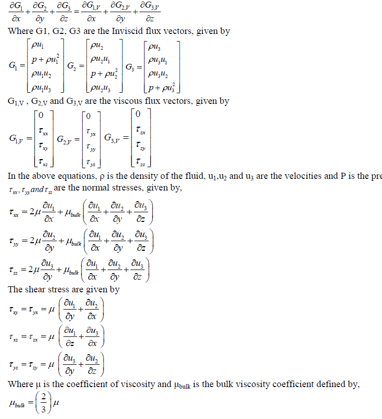
| The governing Navier-Stokes equations for the flow physics considered in this work are written in vector from as, |
 |
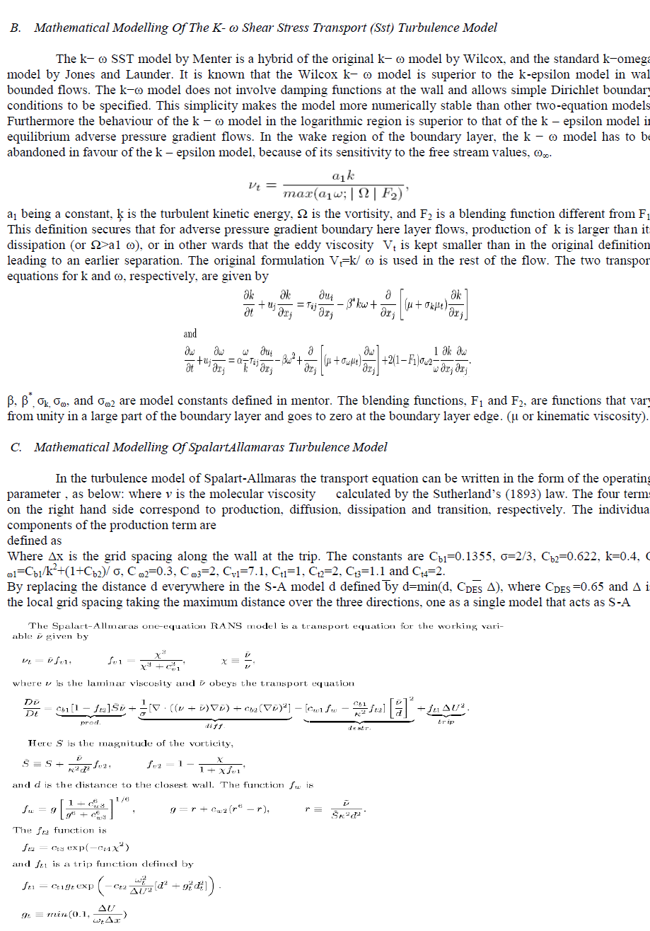 |
| when d << Δ and as a SGS model, when Δ<<d. then SGS model is close to smagorinsky’s in the sense that both make the mixing length proportional to Δ |
| D. Grid independence studies: |
| Both the spalartallmaras turbulence model and k-ω Shear Stress Transport Turbulence models requires a fine resolution mesh in the boundary layer region. The CFD computations need a y plus value of 1 to5 for resolving the laminar sub layer. Table below shows the grid independence studies conducted for and k-ω Shear Stress Transport Turbulence model with transition option. |
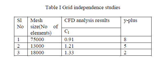 |
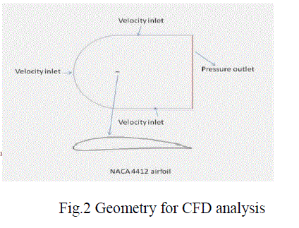
| Experimental values of Cl= 1.38 for an angle of attack of 12 degrees. From the above table it is concluded that grid with 18000 elements is found to be suitable for CFD analysis E. Boundary Conditions: It involves inlet, outlet & wall boundary The velocity components are calculated for each angle attack case as follows. The x-component of velocity is calculated by x ï½ u cosï¡ and the y component of velocity is calculated by y ï½ usinï¡ , where ï¡ is the angle of attack in degrees. The inlet velocity is 43.822 m/sec for a free stream Reynolds number of 3 million and air at STP as the fluid medium The free stream temperature is 300 K which is the same as the environmental temperature. The density of the air at the given temperature is ρ=1.225kg/m3 and the viscosity is μ=1.7894×10⁻⁵kg/ms. for this velocity, the flow can be described as incompressible. This is an assumption close to reality and it is not necessary to resolve the energy equation. Turbulent intensity and viscosity ratio are set to a value of 5 as per the industry practices. Outlet: Ambient atmospheric condition is imposed at outlet. Wall: No slip boundary conditions are imposed. The airfoil surface is treated as wall boundary. A segregated, implicit solver was utilized (Fluent 6.3.26.2006) Calculations were done for angles of attack ranging from 0o to 18°. The airfoil profile, boundary conditions and meshes were all created in the pre-processor Gambit 2.3.16. The pre-processor is a program that can be employed to produce models in two and three dimensions, using structured or unstructured meshes, which can consist of a variety of elements, such as quadrilateral, triangular or tetrahedral elements. Here quadrilateral meshes are used. |
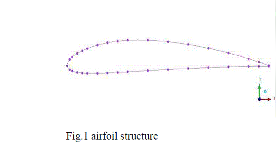
| F. Geometrical Modeling and Grid Generation : |
 |
 |
III. RESULTS AND DISCUSSIONS |
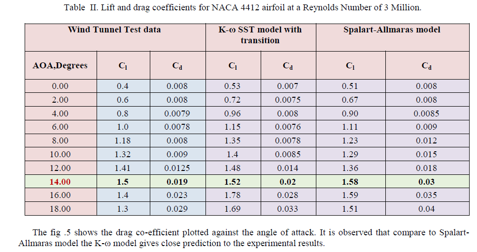
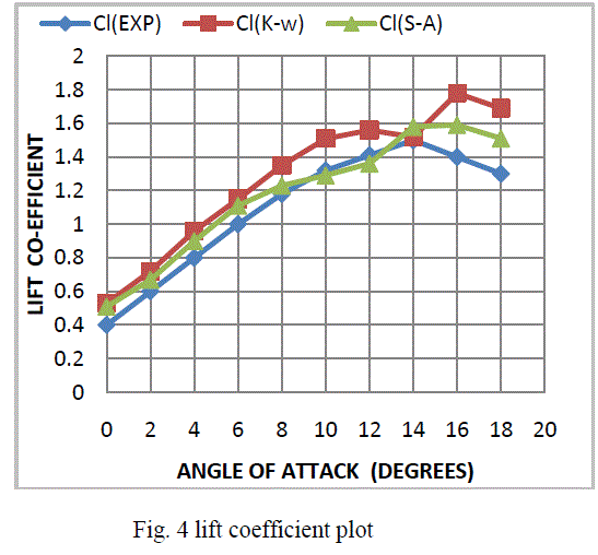
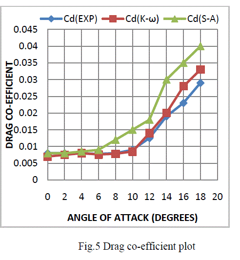
| Table 2 shows the lift and drag coefficients obtained by the wind tunnel test (experimental) results, they are taken from the books “theory of wing sections” by Abott. And this table also contains the lift and drag coefficients obtained by the two different modeling approaches that is K-ω model and Spalart-Allmaras model, comparing these approaches with the wind tunnel results. By comparing the Fluent results with wind tunnel results at different angle of attack from 0-18o K- ω model is well predicted at stalled region. The comparing lift and drag plots are shown in fig 4. Here we observed that shows the lift coefficient plotted against the angle of attack. It is observed that K-ω SST turbulence model with transition capabilities gives close prediction of lift and drag coefficient both in pre stall and post stall region. |
 |
 |
 |
 |
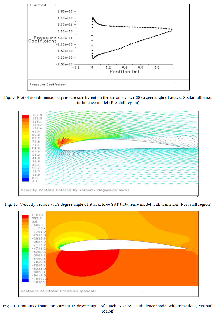 |
| Fig. 9 shows the velocity vectors computed using the K-ω SST turbulence model with transition capabilities(AOA=18 degree), the maximum flow velocity value is 127.9 m/sec. Hence it is observed that K-ω SST turbulence model with transition capabilities is predicting higher flow acceleration near the leading edge of the airfoil and hence relatively higher value of lift coefficient is observed. |
IV. CONCLUSIONS |
| Three dimensional CFD analysis is carried out for viscous incompressible flow around NACA 4412 subsonic airfoil using FLUENT commercial CFD software at a free stream Reynolds number of 3 million. The analysis is carried out with Spalart allmaras turbulence model and K-ω SST turbulence model with transition capabilities Lift and drag coefficients obtained with CFD analyses are compared with the wind tunnel test data available in open literatures. It is observed by these comparisons the two models gives near prediction to the experimental results. It is concluded that K-ω SST turbulence model with transition capabilities gives close prediction of lift and drag coefficient both in pre stall and post stall region. |
References |
|