Research & Reviews: Journal of Agriculture and Allied Sciences
ISSN: E 2347-226X, P 2319-9857
ISSN: E 2347-226X, P 2319-9857
Anuradha Tyagi*, Deepika Punj, Shilpa Sethi
Department of Plant pathology, Bose University of Science and Technology, Faridabad, India
Received: 21-April-2020, Manuscript No. JAAS-23-9583; Editor assigned: 24-April- 2020, Pre QC No. JAAS-23-9583 (PQ); Reviewed: 08-May-2020, QC No. JAAS-23- 9583; Revised: 03-July- 2023, Manuscript No. JAAS-23-9583 (R); Published: 31-July- 2023, DOI: 10.4172/2347-226X.12.2.004
Citation: Tyagi A, et al. Optimization of CNN with LSTM for Plant Classification and Prediction. J Agri Allied Sci. 2023;12:004.
Copyright: © 2023 Tyagi A , et al. This is an open-access article distributed under the terms of the Creative Commons Attribution License, which permits unrestricted use, distribution and reproduction in any medium, provided the original author and source are credited.
Visit for more related articles at Research & Reviews: Journal of Agriculture and Allied Sciences
Plant diseases are a distinct threat to the field of agriculture and plantation around the world. Diseases that are not properly treated will result in a reduction the harvest of the crop. Early identification of the disease is a very important thing. This is to prevent the disease from spreading to other plants. Detection common plant diseases are made by direct observation of each plant. Whereas, the motive behind the research is the find out the disease at the early stage enabling the conservative management technique to initiate the treatment and avoiding the spreading of disease in remaining plants or leaves. The proposed scheme is automatic detection analogy which based on observation using digital image processing supported by the development of visual technology and digital products. The detection of plant disease is based on the leaves got sick due to insects, bacteria or fungi. However, the scheme inculcates the automatic detection of disease in plant and deficiency occurred due to the complex nature of the disease. Therefore, the proposed scheme identifications of type of disease definitions use a gray level comprising CNN (Convolutional Neural Network) and Long Short Term Memory (LSTM) with efficiency any accuracy.
Neural network; Convolution neural network; Long short term memory; Multi layer perceptron
This scheme is proposed to detect the condition of the disease which attacks various categories of plants where there are several diseases from plants such as yellow leaves, black and green young green where the disease is caused by fungus, viruses and factors environment. Where image processing will be used herein leaf condition who has the disease and will conclude the disease owned by plants. On the use of methods in image processing using CNN (Convolution Neural Network) selection of this method due to the research concluded that the classification between MLP and CNN, with variations in parameters, the accuracy of CNN validation is always higher MLP, in another method is LSTM like that says that CNN is better at image recognition visual. Image processing will be taken sample where the sample is used as training data for the health classification of plants.
The leaves of the various plants that will be sampled are the leaves which are healthy and unhealthy leaves are associated with a specific disease with the conclusion of what disease is experienced by categorization so that the handling of the treatment process is done quickly. This last task focused on the symptoms of the diseases of the leaves plants and the prevention measure as conservative management will be rendered [1].
Agriculture or horticulture popularity is evident from the steady and increasing production of plants and fields, so in making this tool it is possible to increase the production of various grains, fruits and vegetables, however, more farmers who are not worried about the spread of disease due to the delay in the process of handling fields. From the data obtained from the ministry of statistics and programmer implementation, it can be seen that the total production of plants from 2008. So that it will form an appropriate environment.
Generally, ornamental plant diseases arise from excessive moisture factors. The rainy season, which results in high humidity, has many cases of emerging diseases, compared to the dry season. The main factor in the prevention of disease attacks is how it can control environmental humidity. Regularly spray with fungicides during the rainy season. Maintain cleanliness in the garden and surrounding area, to prevent waterfalls after rain. Various plants and trees in climatic regions generally live in the soil and form tubers as adaptations in winter. Just as flowers make them different and easily recognizable. These parts of the tribe tend to have high water content organs. Because he can live in low water availability situations. Water is obtained from rain, drops, dew or water vapor in the air. These diseases are then the main purpose of the classification process in this scheme. Here is the data on these diseases that are obtained from processes in the environment that are ideal and ideal for growing them. Few are discussed for the ready reference (literature survey) which is evaluated even in proposed methodology [2].
Spider mites pest
Spider mites pest is a species of mites that is a cultivated orchid pest that generally falls into two main categories, a highly descriptive mite spider mite and avoids confusion with mites. There are other moth species, but they are generally less important. The persistent plant profit mites are the mites (Tetranychus urticae). Spend a profit around the middle. They are active species that can easily be seen roaming the plants. Make a profit for the silk weave they produce, not because they may look like a name by the name of the winter form it is likely that in some cases the red form of the two peaks is actually a global mite, consuming many kinds of plants (polyphagics) and can be easily exported to a wide variety of crops.

Figure 1: Spider mites.
The Figure 1 depicts the effects of spider mites on leaves therefore, the pests (spider mites) that attack the plants will generate the physical hangs on leaves on the surface of leaf especially on the bottom it will be rough and white shades subsequently, which will squeeze the size of leaves and stop the growth of leaves.
Black spot
Black spot on plants leafs responds quickly to something is wrong in their environment. Black spots are one a sign of trouble. The first step in treating black spots on your orchid leaf is to diagnose the problem. Leaf can also indicate bacterial or fungal diseases. Bacteria leaf spots are quite common among leafs and can be aggressive and dangerous. Diseases like fungal disorders and leaf blemishes, especially if the plant is left exposed to humidity and cold. Unless it's valuable, the best approach is throw it away, because the disease is very contagious and will spread from one plant to another from the spark. In Figure 2, it can be seen that the plant has a disease black spot caused by fungal (fungal) [3].

Figure 2: Black spot.
Cercospora
Cerebral leaflet disease of Dendrobium spp. already reported in Florida, Thailand, India and most of the tropics in the world where dendrobium is grown. This happens most often in Florida South and has been significant in the production of dendrobium. Leaf lesions on Dendrobium was first recorded on the leaf surface as dots are pale yellow, with a diameter of 1 mm to 3 mm. Over time, the spot continue to grow in a circular pattern or is irregular and can eventually cover the entire bottom of the leaf. Then the spots become slightly concave and violet with the remaining margins are yellow. After the spots appear on the lower leaf surface, the area is pale yellow as seen on the upper leaf surface. Eventually the spots turn grayish the weight disappeared. Prolonged wet season should be avoided. Chlorothalonil and thiophanate spreading serpentine leaves on orchids in the United States. The result of the test cercospora fungicides performed in 2005 showed that BASF 51604 F (pycadostrobin+boscalid) 38% WG at 340.2 g per 379 L of water and pyraclostrobin 20% WG at 226.8 g per 379 L of water is significantly effective.
Figure 3 depcits signs of the disease comprising oncidium small spots of less than 1mm are found on the underside of the leaves. On Dendrobium yellow dots are 1 cm in diameter. Black spores are found below the leaf surface.

Figure 3: Cercospora on orchids.
RGB color model
The RGB color model is the most commonly used color model on image processing. RGB is a color model of 3 colors: Red, green and blue later various compositions were added to create a new color.
Figure 4 depicts that RGB imagery is made up of three primary color channels red, green and blue. Each RGB color channel can set the color intensity on an 8bit scale or a range of values between 0 to 255. At each pixel of an element's image, create a unity the three colors. As in the 2.6 white image, unity all three are at a maximum value (255,255,255) while for black, the third color combination is at a minimum (0,0,0). Of these three color combinations are found 16 million different colors.

Figure 4: RGB color models.
Neural network
Neural networks are part of the artificial intelligence system is used to process information designed to mimic how the human brain works to solve problems by doing the process of learning through its synaptic change. Neural Network itself is a replica of the nervous system found on the human brain system. In the process, the human brain is made up of the billions of neurons where each of these neurons is connected to tens of thousands of other neurons. A neuron is arranged upward The 3 main components are:
• Dendrites are channels of input signals that are the strength of their connections to the nucleus of a cell is influenced by a weight (Weight).
• The cell body is the place for computing weighted input signals for generates an output signal that is then sent to neurons.
• Axon is the part that sends output signals to neurons other neurons are connected (Figure 5).

Figure 5: Biological neurons in the neural network.
It can be seen in Figure 5, the relationship between neurons biologically and neurons in the neural network. In neural network models, dendrites are represented as inputs that are the information needed by the neural network in solving the given problem.
Whereas the cell body is the site of computational calculation. Subsequently the result of the calculation process performed on the cell body will be output to the output which is the representation of the axon. Generally the artificial neural network has three layers, namely, the Input layer, the hidden layer and the output layer. Here's an explanation of the layer on the NN [4].
Input layer: The input layer contains neurons of an input value that do not change during the training phase and can only change if given a new input value. The neurons in this layer depend on the amount of Input of a pattern.
Hidden layer: This layer never appears until it is called a hidden layer. However, all the processes in the training and recognition phases are carried out in this layer. The amount of this layer depends on the architecture you want to design, but is usually made up of one hidden layer.
Output layer: Output layer function to display system calculation results by activation function on hidden layer based on Received input. Neural networks are defined by three things, which is the pattern of connections between neurons called tissues. Methods for determining the connecting weights are called training/learning/algorithm methods and activation or transfer functions. One of the most popular NN architectures is the multilayer feedforward networks. In general, such networks consist of a number of neuron units as an Input layer, one or more nodes of hidden computational neurons (hidden layers) and a forward nodes layer (output layer direction), layer by layer. This type of network is the result of generalization of a single layer perceptron architecture, so it is commonly referred to as a Multilayer Perceptron (MLP). The reverse propagation (towards the Input layer) occurs after the network generates an output containing an error. During this phase the entire synaptic weight (which has no activation of the zero) in the network will be adjusted to correct for the error correction rule.
For network training, the forward and back propagation phases are repeated for one set of training data and then repeated for several epochs (one session delay for all training data in a network training process) until the Error reaches a certain tolerance limit or zero. The MLP consists of several processing units (neurons) as shown in Figure 6, which are connected and have multiple inputs and have one or more outputs. Perceptron is used to calculate the sum of the values of the weights and inputs of a parameter that is then compared to the threshold value, if the output is greater than the threshold then the output is one and instead is zero.

Figure 6: Multi-layer perceptron structure.
This statement is the result of a formative training process the language is a yes or no statement. Mathematically possible is written with the equation as in Equation 1: The sum of the weights and parameters of the input are: I=wjixiBy: I=Input; xi=input signal wi=weights when I>T then output O=1, with T is the threshold. Training on the perceptron is done by changing the value of the scale so that it meets the needs, is done by comparing the output of JST with its target, process it can be stated as: wbaruji=wlamaji+α (tj-Oj)xi where tj=target, This process is performed on each of the neurons in each layer until the weights are as desired. The initial value of the scale is the small number taken at random. In this final task NN used training and Testing for disease classification. Where once the convolution and sub sampling process is complete, the final process will be combined with NN to obtain the hidden layer value [5].
Convolutional neural network
Convolutional Neural Network (CNN) is a development of the Multilayer Perceptron (MLP) designed to process two dimensional data. Convolutional neural networks are included in the deep neural network type due to their high network depth and are widely applied to imagery data. In the case of image classification, MLPs are less suitable for use because they do not store spatial information from the imagery data and assume that each pixel is an independent feature resulting in poor results. Technically, CNN is a trainer that can be trained and consists of several stages. The inputs and outputs of each level are made up of several common arrays called feature maps. Convolutional neural network itself is a blend of image convolution for feature extraction and neural network for classification. Here is the convolutional neural network architecture network (Figure 7).

Figure 7: Convolutional neural network architecture.
Convolutional Neural Network (CNN) is a development of the Multilayer Perceptron (MLP) included in the neural network type feed forward (not repeated). Convolutional neural network is a neural network that is designed to process two data dimension. CNN is included in the type of deep neural network because of the depth of that network high and widely applied to image data. CNN is used for analyzing visual images, detecting and recognizing objects on images, which is high dimensional vector that will involve many parameters to characterize the network. Broadly speaking, CNN is not too much different from the usual neural network. CNN consists of neurons that have weight, bias and activation functions. Architecture convolutional neural network can be seen in Figure 7. Convolution layer convolutional layer is the layer that first receives the inputted image. This layer performs the convolution process using a filter. This filter is initialized with a certain value (random or using certain techniques such as Glorot) and the value of this filter is the parameter that will be updated in the learning process. This filter will shift to all parts of the image. This shift will produce a dot product between the input and the value of the filter as fully connected layer as fully convolutional layer [6].
According to the LeNet architecture, there are four main layers on a CNN namely convolutional layer, relu layer, subsampling layer and fully connected layer. The following is an explanation of each one. Convolutional layer performs the convolution operation on the output of the previous layer. The layer is the main process underlying a CNN. Convolution is a mathematical term that means applying one function to the output of another function repeatedly. In image processing, the convolution method implements a kernel (yellow box) on all possible offset images as shown in Figure 8. The green box as a whole is the image to be converted. The kernel moves from the top left corner to the bottom right. Equation below is the convolution equation as h(x,y)=f(x,y)*g(x,y). The purpose of convolution on imagery data is to extracts features from input imagery [7]. Convolution will produce linear transformation of the input data according to spatial information in the data. The weight of the layer specifies the convolution kernel is used, so that the convolution kernel can be trained based on the input on CNN (Figure 8).

Figure 8: Convolution operations.
Figure 8 depicts that convolution layer performs convolution operation on output from the previous layer. The layer is a process major underpinning a CNN. Convolution is a mathematical term meaning to apply one function to the output of another function repeatedly. In image processing, convolution that means applying a kernel to the image at all offset possible. The purpose of convolution of imagery data is to extract features from input imagery. Convolution will result in a linear transformation of the input data accordingly spatial information in the data. Weight on that layer specifying the convolution kernel used, so that the convolution kernel can be trained based on the input on CNN.
ReLu layer
ReLu or rectified linear unit layer, this layer can be referred to as thresh holding or just as the activation function in artificial neural networks. With the aim of keeping the results of the convolution process in a positive definite domain. The generated numbers should be positive because of the activation function in the artificial propagating neural network in this study using the relay function. So each value of the negative value convolution proceeds will first go through the ReLu process where the negative value is equal to zero i.e., f(x)=max(0,x). Thereinafter, sub sampling layer is the process of reducing the size of an image data. In image processing, sub sampling is also aimed at increasing position invasion of features. In most CNNs, the subsampling method used is max pooling. Max pooling divides the output from the convolutional layer into smaller grids and then takes the maximum value from each grid to compute the reduced image matrix as shown in Figure 9.
The red, green, yellow and blue grids are the grid groups for which the maximum value will be selected. So the results of the process can be seen in the grid set to the right. The process ensures that the features obtained will be the same even if the image object is translating (shifting) (Figure 9).

Figure 9: Max pooling operations.
According to, use pooling layer on CNN is only intended to reduce the size of the image so it can be easily replaced with a convolutional layer with the same stride as the pooling layer concerned. Fully connected layer is the layer that is usually used in implementation of MLP and aims to transform the dimension of data so that data can be classified linear. Each neurons in the convolutional layer need to be transformed into single data dimension first before it can be put into a fully connected layer. Because it causes data lost spatial information and none the layer can only be implemented at the end of the network. Convolutional 1 × 1 kernel size layer performs the same function as a fully connected layer but still maintaining spatial character of the data.
LSTM (Long Short-Term Memory)
LSTM (long Short-Term Memory) is a type of recurrent neural network that can learn long-term dependencies. LSTMs were presented in, subsequently improved and popularized by other researchers; they cope well with many tasks and are still widely used. LSTMs are specifically designed to address long term addiction. Their specialization is the storage of information for long periods of time, so they practically do not need to be trained.
All recurrent neural networks that are present are in the form of a chain which is repeating modules of a neural network. In standard RNCs, this repeating module has a simple structure, for example, one candidate layer below in Figure 10 depicts the scenario.

Figure 10: ISTM.
Proposed methodology
The process of classification of plant leaves uses CNN along with LSTM in the form of a colored image of plant leaves, then the process of converting color images to images grayish and continued with the leveling process histogram using the histogram method equalization. The next process is filtering use Gabor filters and search values features using GLCM. Then, obtained the feature values in the form of energy to be used as input to the learning process and ELM testing. From the learning process and testing will be obtained the value of accuracy and the speed of the learning and testing process. Schematic classification process using LSTM of plant leaf images the whole is shown in Figure 11.

Figure 11: Proposed architecture using CNN and LSTM.
Image pre-processing
Gray scale image is an image that has gray color intensity (0-255). The use of gray scale images to obtain simple algorithms and reduce the need for complex color image calculations. In the process, a color image consisting of 3 channels, Red (R), Green (G) and Blue (B) is calculated by equation no.1 into one channel, namely gray image.
Gray level convolutional matrix using CNN
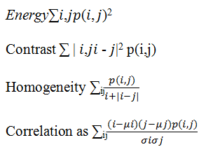
GLCM-CNN is a matrix that describes the frequency of a gray level that appears on a particular spatial linear relationship with the gray level of another pixel. There are two parameters in the calculation of the matrix co relative distances between pairs of pixels measured on the number of pixels and their relative orientation. According to Mokji, et al., there are six texture features that can be used, namely energy, entropy, contrast, variance, correlation and homogeneity. This study only took 4 features that are used to distinguish with other class images, namely energy, contrast, homogeneity and correlation feature equation becomes:
Extreme learning machine
ELM is a feedforward single layer artificial neural network or commonly abbreviated as SLFNs. ELM was first introduced by Huang, Zhu and Siew. There are many types of popular feed forward artificial neural networks which consist of single or multi hidden layers such as learning gradient bases, for example the back propagation method for multi neural networks. However, the learning is very slow than expected, this is because all the parameters given must be determined manually and iterative tuning is needed for each parameter. In the ELM method each parameter is randomly given without iterative tuning so as to produce a fast learning speed. The ELM method has a structure similar to SLFNs, but has a different computational model. Mathematically, ELM is modeled as follows:
• The training set X and sample target T, where:
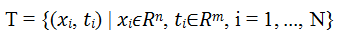
• The number of features of the sample is symbolized by n; the activation function is symbolized by g (x)
• The number of nodes in the hidden layer is symbolized with L
• Input weight vector values (W) and hidden nodes bias (b) randomly determined
From the previous explanation, the calculation mathematically is as follows:
Calculate the output of the hidden layer
• H=H (g (w.x+b)
• Calculate the output weight (β)
• Calculate the value of output Y
• Y=HTβ
LSTM
Using solitary encrusted neural networks in the midst of the sigmoid establishment function excluding candidate layer (it takes Tanh as instigation utility). These gates primary take contribution vector dot (U) in totaling to earlier hidden state. Dot (W) then concatenate them and affect establishment function, in conclusion, these gates generate vectors (between 0 and 1 for sigmoid, -1 to 1 for Tanh) so we get four-vectors f, C, I, O for every time step is Ct=Ct-1*ft where the current segmoid state Ct we calculate new segmoid state from input state and C layer will be Ct=Ct+(It*Ct) for classification and prediction.
The data used in this study which is the digital image of plant leaves obtained from public database. Data The plant leaf image has a size of 500 × 375 RGB pixels (red, green, blue) as many as 32 plant classes with data each class varies. Total data namely 1798 plant leaf imagery. Plant leaf imagery used in this research is original image without pre used shown in the form Figure 12 represents examples of plant leaf imagery data used in this study [8].

Figure 12: Plant leaf image.
Experimental results
Using data as many as 1,797 plant leaf imagery from 32 different classes. The whole data is divided into two groups namely training data and test data. The distribution of training data and test data is varied. 10% training data and 90% test data, 30% training data and 70% test data, 50% training data and 50% test data, 70% training data and 30% test data and 90% training data and 10% test data, respectively. In addition, experiments were performed using 100% training data and took 10 leaf images from each class used for the test data (Table 1) [9].
| No | Percentage sharing data | Sigmoid | Sinusoid | ||||
|---|---|---|---|---|---|---|---|
| AB (%) | AU (%) | WB (s) | AB (%) | AU (%) | WB (s) | ||
| 1 | 10% DL, 90% DU | 99.5 | 72 | 0.4 | 99 | 68 | 0.1 |
| 2 | 30% DL, 70% DU | 93.9 | 86 | 0.5 | 93 | 83 | 0.5 |
| 3 | 50% DL, 50% DU | 90.7 | 86 | 0.8 | 91 | 85 | 0.8 |
| 4 | 70% DL, 30% DU | 89.9 | 87 | 1.1 | 90 | 85 | 1.8 |
| 5 | 90% DL, 10% DU | 90.2 | 83 | 1.5 | 89 | 84 | 1.5 |
| 6 | 100% DL, 10% DU | 89.9 | 92 | 1.7 | 89 | 92 | 1.8 |
Note: DL: Training Data; DU: Test Data; AB: Learning Accuracy; AU: Testing Accuracy; WB: Training Time
Table 1. Experimental results with training data and test data varies.
Data sharing is done to see the level the accuracy of each different amount of data with sigmoid and sinusoid activation functions. Percentage of accuracy in learning and testing is indicated by the results of the classification true for any trained or tested imagery data into the appropriate plant class, versus with the amount of training data or test data that set. Table 1 shows the results of accuracy leaf imaging data learning and testing plants with a value of hidden node 95. One of the attributes that influences accuracy LSTM learning and testing is a sum hidden node specified. Table 2 shows test results with the number of hidden nodes varies [10].
| S. no | Amount of hidden nodes | Learning accuracy | Accuracy testing |
|---|---|---|---|
| 1 | 30 | 74.90% | 73.40% |
| 2 | 35 | 79.30% | 78.30% |
| 3 | 40 | 80.20% | 81.90% |
| 4 | 45 | 83.20% | 81.70% |
| 5 | 50 | 84.70% | 81.92% |
| 6 | 55 | 85.90% | 82.20% |
| 7 | 60 | 87.10% | 84.40% |
| 8 | 65 | 88.40% | 85.90% |
| 9 | 70 | 89.00% | 85.60% |
| 10 | 75 | 88.80% | 86.90% |
| 11 | 80 | 89.40% | 86.30% |
| 12 | 85 | 90.10% | 86.70% |
| 13 | 90 | 91.30% | 86.90% |
| 14 | 95 | 90.60% | 86.70% |
| 15 | 100 | 91.50% | 85.60% |
| 16 | 105 | 91.50% | 87.60% |
| 17 | 110 | 92.30% | 87.20% |
| 18 | 115 | 92.00% | 88.70% |
| 19 | 120 | 91.00% | 87.40% |
| 20 | 125 | 92.70% | 88.70% |
| 21 | 130 | 92.90% | 88.90% |
Table 2. Experiment with hidden nodes.
In the experiments conducted, there were several mechanisms for testing the classification of plant leaf images using CNN and LSTM methods. Activation functions used are sigmoid and sinusoid. From the experiments that have been carried out obtained the value of accuracy and learning time. Figure 3 shows a graph of the results of the experiments that have been carried out [11]. Table 1 shows the results in the form of accuracy values obtained in accordance with the amount of data sharing that has been done. In the experiments using the binary sigmoid activation function with the division of training data and test data of 10% and 90%, the learning accuracy value was 99.4% and the test accuracy value was 71.75%. In the 30% and 70% data sharing, the learning accuracy value decreased by 93.9% but the value of testing accuracy increased by 85.5%. In the next experiment 50% of the data sharing accuracy of learning is 90.7% and 89.9% and has increased the value of testing data accuracy of 85.8% and 86.9%, but a slight decrease in training 90% and testing 82.7%. In addition to all the results described there are additional experiments that use 100% of data for training and take 10 data from each of the results of the learning accuracy of this experiment that is 89.9% and testing accuracy of 91.5%. Unlike the experimental mechanism using the sinusoid activation function get a higher accuracy value than the binary sigmoid activation function. From several experiments using the percentage of training data and different test data obtained values of learning accuracy sequentially of 98.9%, 92.8%, 90.6%, 90.1%, 88.5% and 91.5% and the value of testing accuracy of 67.6%, 83.1%, 84.9%, 85.2%, 83.5% and 91.5%. The values obtained indicate that the greater number of training data samples will increase the value of learning accuracy. In addition to the number of input data samples that affect the accuracy of learning the selection of activation functions also affect the accuracy value (Figure 13) [12].

Figure 13: Graph the results of experiments with variation in the amount of data.
The next experimental mechanism uses the training data distribution and the 0.3 sinusoid test data of 90 and the various hidden node values. The use of various hidden node values aims to see the effect of the number of hidden node values on the level of accuracy of learning and testing of the proposed methods [13,14]. Figure 13 shows the graph of the experimental results using various hidden node values. Learning accuracy increases when the value of hidden node increases from 30, 35, 40, 45 and 50 but decreases in hidden node 55 and increases in the next hidden node value. The same thing happened with testing accuracy. The highest accuracy value is obtained when the hidden node value of 130 is 92.9% for learning accuracy and 88.9% for testing accuracy [15]. The higher the hidden node value, the higher the accuracy value. Consequently, to find the disease range or the infection range on the leaves the calculation based on experimental results with training data and test data varies i.e., Description: DL: Training data, DU: Test data, AB: Learning accuracy, AU: Testing accuracy, WB: Training time using sigmoid and sinusoid is evaluated vide this proposed equation (Table 3).
Disease percentage=(Sigmoid learning accuracy*sinusoid testing accuracy)/100-(Sigmoid testing accuracy*sinusoid testing accuracy)/100.
Percentage of disease incidence host response:
0%-10%: Resistant 11%-30%: Moderately resistant 31%-60%: Moderately susceptible 61%-100%: Susceptible
| S. no | Percentage sharing data | AB (%) | AU (%) |
WB (s) |
AB (%) |
AU (%) |
WB (s) |
Disease in percent | Status |
|---|---|---|---|---|---|---|---|---|---|
| 1 | 10% DL, 90% DU |
99.5 | 72 | 0.4 | 99 | 68 | 0.1 | 49.545 | Moderately susceptible |
| 2 | 30% DL, 70% DU |
93.9 | 86 | 0.5 | 93 | 83 | 0.5 | 15.947 | Moderately resistant |
| 3 | 50% DL, 50% DU |
90.7 | 86 | 0.8 | 91 | 85 | 0.8 | 9.437 | Resistant |
| 4 | 70% DL, 30% DU |
89.9 | 87 | 1.1 | 90 | 85 | 1.8 | 6.96 | Resistant |
| 5 | 90% DL, 10% DU |
90.2 | 83 | 1.5 | 89 | 84 | 1.5 | 10.558 | Resistant |
| 6 | 100% DL, 10% DU |
89.9 | 92 | 1.7 | 89 | 92 | 1.8 | -4.629 | Resistant |
Table 3. Results comprising the status based on calculation based on disease in percent using CNN.
Based on test results on test data image of plant leaves can be concluded that image classification of plant leaves using CNN-ELM along with LSTM method is successfully carried out by value 92.9% learning accuracy and testing accuracy of 88.9%. The test results are determined by the number training data used. More and more data practice it will increase the value of accuracy the test. Determination of the number of hidden nodes influential great in producing accuracy values. Results experiments show that the hidden node value of 130 produces the best accuracy value. Thereinafter the Table3 depicts the disease status based on percentage of effectiveness achieved for detailed elaboration.
[Crossref] [Google Scholar] [PubMed]