ISSN ONLINE(2319-8753)PRINT(2347-6710)
ISSN ONLINE(2319-8753)PRINT(2347-6710)
S.M.Meena1*, V.S.Velladurai2
|
| Related article at Pubmed, Scholar Google |
Visit for more related articles at International Journal of Innovative Research in Science, Engineering and Technology
Dimensionality reduction is vital in many fields, and alignment-based methods for nonlinear dimensionality reduction have become popular recently because they can map the highdimensional data into a low-dimensional subspace with the property of local isometry. However, the relationships between patches in original high-dimensional space cannot be ensured to be fully preserved during the alignment process. In this paper, we propose a novel method for nonlinear dimensionality reduction called local coordinates alignment with global preservation. We first introduce a reasonable definition of topology-preserving landmarks (TPLs), which not only contribute to preserving the global structure of datasets and constructing a collection of overlapping linear patches, but they also ensure that the right landmark is allocated to the new test point. Then, an existing method for dimensionality reduction that has good performance in preserving the global structure is used to derive the low-dimensional coordinates of TPLs. Local coordinates of each patch are derived using tangent space of the manifold at the corresponding landmark, and then these local coordinates are aligned into a global coordinate space with the set of landmarks in low-dimensional space as reference points. The proposed alignment method, called landmarks-based alignment, can produce a closed-form solution without any constraints, while most previous alignment-based methods impose the unit covariance constraint, which will result in the deficiency of global metrics and undesired rescaling of the manifold. Experiments on both synthetic and real-world datasets demonstrate the effectiveness of the proposed algorithm.
Keywords |
| Isometric mapping, manifold learning, nonlinear dimensionality reduction, tangent space. |
INTRODUCTION |
| THE PROBLEM of dimensionality reduction arises in many fields, such as machine learning, neural computation, data mining, and pattern recognition. The task of dimensionality reduction is to recover meaningful low-dimensional structures hidden in high-dimensional data. An example might be a set of pixel images of an individual’s face observed under different poses and lighting conditions; the task is to identify the underlyingvariables (pose angles, direction of light, etc.,) given only the high-dimensional pixel image data. In manycases of interest, the observed data are found to lie on an embedded submanifold of the high-dimensional space. The degrees of freedom along this submanifold correspond to the underlying variables. In this form, the dimensionality reduction problem is known as manifold learning. Spectral methods have recently emerged as a powerful tool for dimensionality reduction and manifold learning. These methods are able to reveal lowdimensional structure in highdimensional data from the top or bottom eigenvectors of specially constructed matrices. To analyze data that lie on a low-dimensional submanifold, the matrices are constructed from sparse weighted graphs whose vertices represent input patterns and whose edges indicate neighborhood relations. The main computations for manifold learning are based on tractable polynomial-time optimizations, such as shortest path problems, least squares fit, semidefinite programming, and matrix diagonalization. Principal component analysis (PCA) [1] and metric multidimensional scaling (MDS) [2] are simple spectral methods for linear dimensionality reduction. Recently, from the viewpoint of manifold learning, some new linear methods have been proposed, such as locality preserving projection [3], neighborhood preserving embedding [4], local discriminant embedding [5], unsupervised discriminant projection [6], and orthogonal neighborhood preserving projections [7]. These methods are successfully only when the data manifold is linear. Recently, progress has been made in developing efficient algorithms to be able to learn the low-dimensional structure of nonlinear data manifolds. These proposed methods include isometric mapping (Isomap) [8], [9], locally linear embedding (LLE) [10], [11] and its variations [12]–[15], Laplacian eigenmap (LE) [16], Hessian eigenmap [17], local tangent space alignment (LTSA) [18], maximum variance unfolding (MVU) [19], diffusion map [20], [21] and semisupervised generalized discriminant analysis [22]. The following |
| two strategies are shared in most of these algorithms |
| 1) exploiting the local geometry around each data point; and |
| 2) mapping the manifold nonlinearly to a lower dimensional space based upon the learned local geometric information. Of course, these algorithms are different in the performance of local information xtraction and global embedding. For example, LLE extracts the linearity by representing each point as a linear combination of its neighbors and then determines a low-dimensional embedding that preserves the locally linear combination structures. LLE is computationally efficient because it involves only sparse matrix computations which may yield a polynomial speedup; however, it neglects the global properties of the dataset. As a result, if two data points in the high-dimensional space are remote, LLE cannot ensure their corresponding data points in a lower dimensional space be remote. Some methods, such as Isomap, distance penalization embedding (DPE) [23], etc., try to keep both local and global properties; however, they have deficiencies to some extent. Isomap estimates the pairwise geodesic distance based on Euclidean distances between neighbors and then maps the high-dimensional points into a lower dimensional Euclidean space by preserving the geodesic distances. The derived geodesic distance matrix is inaccurate. In most cases, distances between neighbors are slightly smaller than the true value, and distances between far away data points are always larger than true. As a result, Isomap cannot derive local structure well. In addition, the mechanism of keeping the distances is effective only for globally isometric manifolds. For those manifolds that cannot be isometrically mapped to a lowerdimensional Euclidean space, Isomap may fail. DPE tries to make the neighboring points to be still in the neighborhood and the remote points still to be remote by penalizing the distances. However, the penalization on local distances, as a looser constraint on neighborhood than constraints such as isometry and linear reconstruction, may distort the true structure of the neighborhood. Sun et al. [23] proposed a two-step framework for nonlinear dimensionality reduction: in the first step, DPE is used to obtain the embedding of part of data points, and, in the second step, an additional constraint on the neighborhood relationships is imposed to refine local description by employing semisupervised manifold learning algorithms. However, the algorithm is very sensitive to parameters, and the parameter selections rely on some kind of performance evaluation of the dimensionality reduction algorithm, which is still an open problem. By combining the ideas of MVU and LE, Wang and Li [24], [25] proposed a manifold method that unfolds the dataset by maximizing the global variance subject to the proximity relation preservation constraint originated in LE. However, the method brings undesirable concentration on the boundary of the lowdimensional representation and its performance is very sensitive to parameters. Wang et al. [26] proposed locality-preserved maximum information projection (LPMIP) which considers both within locality and between locality in the processing of manifold learning. However, LPMIP is essentially linear and cannot provide reliable and robust solutions to nonlinearity distributions. Since Zhang et al. [18] proposed LTSA, which uses PCA to construct an approximation for the tangent space at each data point, and these tangent spaces are then aligned by a set of optimized affine transformations to give the global embedding, alignment technology has been a concern to many manifold learning researchers. The main advantage of alignmentbased algorithms is that they can map the high-dimensional data into a lowdimensional subspace with the property of local isometry. LLE and LE are reformulated, respectively, using alignment technology in [27] and [28]. Three key issues in manifold learning determine the effectiveness of alignment-based algorithms. One issue is how to find a finite open cover of the manifold. A commonly used method is to constitute a neighborhood for each data point, and all of these neighborhoods naturally constitute a finite open cover of the manifold [18], [29]. However, the patches obtained this way are heavily overlapped and many of them can be ignored with little effect on manifold learning. To overcome it, Li [30] uses a greedy algorithm to combine a number of these patches into a larger patch. However, it is argued that the resulting patches will have the same fixed size and cannot be suitable to deal with the data nonuniformly sampled from a manifold [31]. In [32], a maximal linear patch (MLP) is first constructed for each data point under a geodesic distance constraint, and then a minimum subset of these MLPs is selected as a finite open cover of the manifold. The second issue is local isomorphic mapping. At present, PCA is often used to get the local coordinates of manifold [18], [30]. The last but not least issue is that of alignment, i.e., aligning the local coordinates of the manifold in the d-dimensional Euclidean space to form the global coordinate of the manifold. The most commonly used methods are the so-called global alignment methods. These methods align all local coordinates of the manifold, all simultaneously, by solving an eigenvalue problem [18], [27], [28], [30]. However, the large data size will lead to a large-scale eigenvalue problem which is hard to solve even for the state-of-the-art eigensolvers [33]. Moreover, the normalization constraints make them fail to preserve geodesic distances. Additionally, some progressive alignment methods [34], [35] select the local coordinate of a patch as the base local coordinate and then progressively expand the base local coordinate by aligning other local coordinates to the base local coordinate patch by patch until the base local coordinate becomes the global coordinate of the manifold. These progressive algorithms cannot ensure the minimum alignment error during each alignment, and the alignment errors will be accumulated and propagated during the process of progressive alignment. In this paper, we propose a new method for nonlinear dimensionality reduction, called local coordinates alignment with global preservation (LCA-GP). Compared with the existing methods, our method has the following features. |
| 1) LCA-GP introduces a novel concept of topologypreserving landmarks (TPLs), which can preserve the global topological structure of manifold and construct a finite open cover of the manifold, i.e., a set of overlapped linear patches. The global nonlinear data structure is then represented by a collection of local coordinates as wellas the set of TPLs. |
| 2) LCA-GP learns the local manifold structures on a set of overlapping linear patches rather than on the neighborhood of each data point, which will reduce the redundancy. |
| 3) LCA-GP aligns the local coordinates into a global low-dimensional coordinate space by landmarks-based alignment (LA), which can well preserve both the local geometry and the global structure of the manifold. |
| 4) LCA-GP only needs to solve a linear system rather than an eigen problem with a unit covariance constraint as most spectral methods do. This kind of constraint will result in the deficiency of global metrics and undesired rescaling of the manifold. |
| 5) LCA-GP approximately learns a nonlinear invertible mapping function in a closed form. Thus, the mapping can analytically project the test data points. This paper is organized as follows. Section II describes the motivation and basic ideas of the proposed LCA-GP. The detailed implementation of LCA-GP along with theoretical analysis is given in Section III. Section IV presents results of experiments on both synthetic and real-world datasets. Section V concludes this paper with directions for future work. |
MOTIVATION AND BASIC IDEAS |
| Most spectral methods for nonlinear dimensionality reduction try to preserve the local geometry around each point |
| and solve optimization problems to obtain the global embedding. The global structure cannot be fully preserved by these methods due to their ignorance of the global properties of manifold. Moreover, the unit covariance constraint is imposed to obtain a unique solution, and the optimization problem turns into an eigenvalue problem. However, the imposed constraint should bring undesired relations among components of the embedding coordinates, which will result in the deficiency of global metrics and undesired rescaling of the manifold, as also pointed out in [31]. The question is how to preserve global structure as well as local geometry and avoid imposing the unit covariance constraint during solving the optimization problem. As described in the introduction, some works attempted to address all or part of these problems; however, each of them has some disadvantages. Inspired by the two-step framework for dimensionality reduction proposed by Sun et al. [23], we can select a set of representative points and use some global algorithm for dimensionality reduction to obtain lowdimensional coordinates of these points in the first step, and then develop some manifold learning algorithm, in which the optimization problem under the constraint of a set of representative points can be transformed into a problem of solving linear system, to derive the embedding of all data points. There are two issues in the first step: one involves the selection of representative points and the other is to get the embedding coordinates of these selected points. The focus of this paper is the first issue. Representative data points, which we call landmarks, are selected from datasets that lie on an embedded manifold of the highdimensional space. These landmarks should preserve the topology of the manifold and should be capable of learning the structure of certain curved manifolds. A criterion to test whether a landmark set can accurately and reliably represent the manifold was proposed in [36]. The criterion ensures that the individual Voronoi cells generated by the landmarks in the ambient space do not intersect the manifold at distant locations but it leaves out to ensure the linear structure of each cell. In [23], the centers of those neighborhoods that constitute a minimum set that cover the dataset are taken out as landmarks. The landmarks found in this way depend largely on the distribution density rather than some topological structurerelevant factors, such as curvature and so on. |
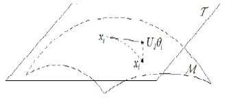 |
| Fig. 1. Illustration of manifold M, tangent space T at a landmark xl, and projection of the vector xi − xl on T , Ul θi, where θi is the coordinate of Ul θi under Ul , i.e., the local coordinate of a point xi . |
| In this paper, we find a set of landmarks that not only ensures that for new test points the closest landmark in terms of Euclidean distance is also close in terms of geodesic distance on the manifold [36] but also can construct a set of corresponding neighborhoods such that these neighborhoods are linear and overlapped with each other and all together cover the whole dataset. Specifically, for the latter, the approximation error of the point to the tangent space at the landmark is small enough. Consider the linear structure of a neighborhood of landmark xl = f (yl), where f : Rd → RD, d << D, which can be characterized by the tangent space of the manifold at xl . |
| A neighbor xi = f (yi ) of xl can be represented by xi = xl + J f (yl)(yi − yl) + ε(yi , yl) (1) where J f (yl) is the Jacobian matrix of f at yl , whose columns span the tangent space, and ε(yi , yl ) is a second order term of yi − yl , which measures the approximation error of xi to the tangent space. Consider that the second-order term should be small, i.e., the first-order term should be close to xi − xl .With the assumption that the manifold is smooth enough and dataset is dense enough, we have |
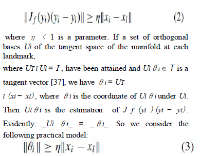 |
| as a criterion to test whether a set of landmarks can reliably represent the manifold (see Fig. 1 for an illustration). Based on this criterion, in this paper we give a new concept of TPLs and propose an adaptive TPL selection method. The second step is about the landmark-constrained manifold learning algorithm. As described in the introduction, three key issues in manifold learning determine the effectiveness of alignment based algorithms. If there are a set of TPLs as well as their lowdimensional coordinates, landmarks-based methods on the three issues are proposed. At first, each data point is the neighbor of its two nearest landmarks, and the are approximately linear. Then tangent space of manifold at the landmark point, instead of at the mean point of patch, is used to derive the local coordinates of each patch. Finally, we take the low-dimensional coordinates of landmarks as constraints and transform the optimization problem in alignment into solving a linear system to obtain the last embedding. We call this LA. Briefly, the novelty of the proposed LCA-GP is twofold: the concept of TPLs and the LA method, which lead to several highlighted characteristics as described in the introduction part. |
LCA-GP |
| In this section, we first introduce the concept of TPL,and the proposed method for TPL construction, as well as finite open cover construction. Then, the learning procedure of LCA-GP is presented in detail, including obtaining the global coordinates of TPLs, the construction of local model, and the landmarks-based alignment, i.e., the LA method. Finally, theoretical analyses of LCA-GP and comparisons of LCA-GP with other relevant methods are discussed. |
A. TPLs and Finite Open Cover |
| Landmarks introduced in our algorithm not only contribute to preserving the global properties of the dataset and constructing a proper finite open cover of manifold but also ensure to allocate the right landmark to a new test point. The principal insight of the qualified set of landmarks lies in three criteria: |
| 1) topological structure of manifold is well preserved by landmarks; 2) each data point is the neighbor of its two nearest landmarks, and the neighborhood of each landmark constitutes a patch, which spans a near linear subspace; and 3) for new test points, the closest landmark in terms of Euclidean distance is also close in terms of geodesic distance on the manifold. Those landmarks satisfying the above three criteria are called TPLs. |
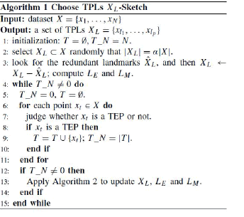
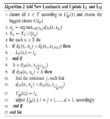
| The first two criteria can consider that the approximation errors of each data point to the tangent space at its two nearest landmarks are small enough. As to the third one, we use the method proposed in [36]. Specifically, to each data point, the nearest landmark measured with neighborhoods of all landmarks constitute the finite open cover of the manifold. We take each neighborhood as a patch . There should be common points in adjacent patches, and all patches Euclidean distance is the nth nearest one measured with geodesic distance, where n ≤ d+1 and d is the intrinsic dimension of the manifold. Suppose X = {x1, . . . , xN } is a set of N data points, where xt ∈ RD, t = 1, . . . , N, which are assumed to be drawn from a probability density, which is supported on a d-dimensional manifold M embedded in RD, where d < D; and the landmarks will be chosen from X. Let the landmarks’ indices be L = l1, l2, . . . . Then XL is the set of landmarks, and xli represents the i th landmark. A sketch of finding TPLs algorithm is given in Algorithm 1. The parameter α is the proportion of alternative initial landmark points. We set α as 0.05 without careful selection because it makes little difference to the result due to the following step of removing redundant landmarks. If the approximation error of one landmark xlR to the tangent space at one of the other landmarks is small, xlR is thought to be redundant and will be removed from the set of landmarks. The set T contains all of the topological error points (TEPs) corresponding to the current set of landmarks. The matrices LE and LM will be described in the next paragraph. The goal of the algorithm is to find a set of landmarks. These landmarks can reliably represent the manifold, and can be used to construct linear patches. These landmarks also can generate individual Voronoi cells in the ambient space including both xt and xL j M(xt ), j = 1 or 2 does not span a near linear subspace. However, the problem of how to define the criterion for enough on an unknown manifold is inherently ill-posed. According to the analysis in the above section and in [36], we thus turn to defining element of the vector LE in Algorithm 1 is [LE (xt )], and the tth column of the matrix LM is [L1 M(xt ) ... L(d+1) M (xt )]T . We denote the inverse map for L j M(xt ) as Cellj M (l) = {xt |L j M(xt ) =l}. The meaning of the “cell map” is as follows: given a landmark, find the data points that take this landmark as the j th landmark. TEP indicates that the projection error of xt onto the tangent Euclidean distance in RD, and dM(.,.) stand for the that do not intersect the manifold at distant locations. If there are some TEPs, new landmarks should be added. Topological error points: let dE (.,.) stand for the |
 |
 |
| geodesic distance in M (we derive the geodesic distance between two data points using the algorithm in [8]). Given xt ∈ M, LE (xt ) denotes the index of its nearest landmark with respect to dE(ãÃÆû, ãÃÆû), and L j M(xt ) denotes the index of its j th nearest landmark with respect to dM(., .) on M. The tth space of manifold at xL1 M(xt ) or xL2 M(xt ) is large, or xt and xLE(xt ) are distant enough from each other such that the connection between them makes a short-circuit of that manifold. If only given the first criterion, xL1 M(xt ) will be enough. Given the second criterion, as a res ult, both xL1 M(xt ) and xL2 M(xt ) are considered here. Then, the question is how to test whether xt is a TEP. One needs to judge that whether the projection error of xt onto the tangent space of manifold at xL1 M(xt ) and xL2 M(xt ) is large enough such that one patch heuristics. |
| 1) Given a data point xt , we find the number n such thatLE (xt ) = Ln M(xt ). Compute the xt ’s local coordinates in the tangent space of manifold at xL j M(xt ) , θ j t , j = 1, 2. If _θ j t _/_xt −xL j M(xt ) _ < η, j = 1 or 2, or n > d+1, xtis taken as a TEP, where η is the parameter to determine the local linearity. Redundant landmarks can also be removed by this criterion (see step 3 in Algorithm 1). Specifically, if _θ L mn _/_xlm xln _ > η, where θ L mn is xlm s local coordinate in the tangent space of manifold at xln, then xlm is redundant and will be removed. We go through landmarks in a random order and remove the redundant ones sequentially. To eliminate the TEPs, new landmarks should be added. A simple solution is to choose a new landmark among those TEPs (step 13 in Algorithm 1). We first cluster TEPs, i.e., all x ∈ T , according to their L1 M(x). The second step is to choose a point in the biggest cluster C(lm) as the new landmark xlq by picking up the one that is the farthest from xlm. When a new landmark xlq is acquired, we need to update LE (xt ) and L j M(xt ), j = 1, . . . , d + 1 for all xt ∈ X (step 13 in Algorithm 1). The procedure is shown in Algorithm 2. Fig. 2 shows the unevenly sampled S-curve and the chosen landmarks for it by three methods, i.e., method in [36], method in [23], and our method. There are too few landmarks to preserve the global structure in Fig. 2(b). In Fig. 2(c), the landmarks are distributed unevenly as the origin data points do. There are too few landmarks to preserve the global structure in the sparse part and too many landmarks which will result in redundancy in dense part. In contrast, the TPLs found by our method can reflect the structure of manifold better [see Fig. 2 (d)]. Since the set of TPLs has been settled, the construction procedure for overlapping patches is straightforward. Suppose XL = {xl1, . . . , xl p } is the set of TPLs. There are p overlapping linear patches corresponding to these landmarks. The i th patch |
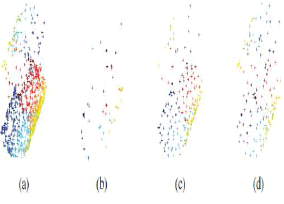 |
| Fig. 2. Synthetic S-curve dataset. (a) 800 points sampled unevenly on S-curve manifold. (b) 41 landmarks chosen by method in [36]. (c) 173 landmarks chosen by method in [23]. (d) 138 TPLs. (For interpretation of the references to color in these figures, the reader is referred to the online version of this paper.) is |
| B. Global Coordinates of TPLs |
| Some existing methods, such as MVU [19], Isomap [8], diffusion map [20], RML [31], and DPE [23], etc., which have good performance in preserving the global structure, can be used to derive the low-dimensional coordinates of TPLs. Because this point is not the focus of this paper and in view of the Isomap as a well-known classical algorithm, we chose an improved Isomap called topologically constrained isometric embedding (TCIE) proposed in [38] recently. All data points are used in the step of looking for the boundary points, and then TCIE is run on TPLs. We call it the global TCIE on landmarks. Suppose X = _x1 ãÃÆû ãÃÆû ãÃÆû xN _ is the matrix of Ddimensional data, and XL = _xl1 ãÃÆû ãÃÆû ãÃÆû xl p _ is the matrix of p landmark points which are the output of Algorithm 1. Global TCIE on landmarks (G-TCIE) has four steps. 1) Compute the N × N matrix of geodesic distances |
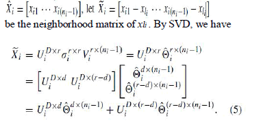
| DM = dM(xi , x j ). (In fact, this step has been done in Algorithm 1 in order to obtain LM.) Then, the geodesic distance matrix of landmarks is DL = ST L DMSL, where SL is a 0–1 data selection matrix such that XL = XSL . 2) Detect the boundary points ∂M of the data manifold. (Refer to [38].) 3) Detect a subset of consistent distances according to either (criterion 1) ïÿãP 1 = {(li , l j ) : cM(xli , xl j ) ∩ ∂M= ∅} where cM(xli , xl j ) is the geodesic connecting xli and xl j , or (criterion 2, we use this criterion in our experiments) ïÿãP 2 = {(li , l j ) : dM(xli , xl j ) ≤ dM(xli , ∂M) + dM(xl j , ∂M)} where dM(x, ∂M) = in fx_∈∂MdM(x, x_) denotes the distance of x from the boundary of M. 4) Solve the MDS problem for consistent pairs only Y ∗ L = argmin YL_ li<l j wi j (dli l j (YL ) − dM(xli , xl j ))2 where wi j = 1 if (li , l j ) ∈ ïÿãP and wi j = 0 otherwise By (4), we obtain p overlapping patches corresponding to p landmarks. We denote these patches as X1. . . . . X p, and the i th patch consists of a set of ni data points in X. For a patch Xi with ni data points, where the corresponding landmark is xli and the matrix of the other ni − 1 points is |
 |
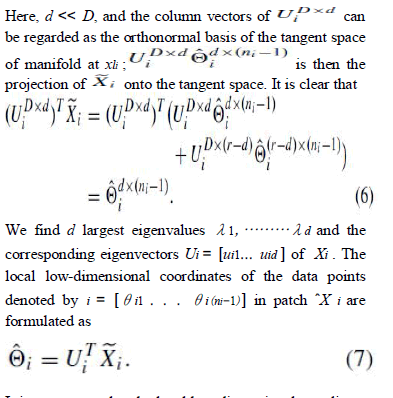 |
| It is easy to see that the local low-dimensional coordinate of xli is a d-dimensional zero vector. Then we obtain the local coordinates of the whole patch i . Because the approximation errors of the data points in eacpatch to the tangent space at the corresponding landmark are small and these data points are thought to reside on a local linear space, the usage of the coordinates of data points on the tangent space of the manifold at landmark to obtain the local representations becomes reasonable in our work. Let Yˆ = [y1 . . . yN−p]be the global coordinates of all input data points excluding p landmark points. i represents the local geometry of the manifold in patch Xi , and Yˆ can be constructed by aligning all patches through translation, rotation, and scaling with landmarks as reference points, called LA. Formally, let Yi represent the global coordinate of i in Rd . The low-dimensional coordinate of the i th landmark derived by TCIE is yli, and let yli ∈ Yi , correspondingly, its local coordinate is θli , θli |
| ∈ i . As mentioned before, θli is a d-dimensional zero vector. Firstly, each patch is translated such that the corresponding landmark point θli meets yli . In order to express easily, we can assume the i th landmark yli to be the ni th point in its patch Yi . Taking out yli from Yi , we have Yˆi = [yi1 . . . yi(ni−1)]. Subtracting yli from all the data points in Yˆi , we have where _ = _1 ãÃÆû ãÃÆû ãÃÆû 1_T . Next we rotate and scale the patch to |
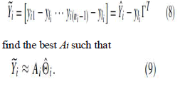 |
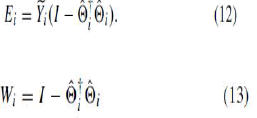
| In (9), Ai represents a linear transformation matrix. The alignment error of local representations Ei can be expressed as |
| In order to minimize the Frobenius norm _Ei_, we need to solve Ai using a least-squares fitting method. The solution is given by |
| we can obtain |
| Let |
 |
| and Si be 0–1 data selection matrix such that Yˆi = Yˆ Si . The squared alignment error of the data in patch Xi can be written as |
| From the global view, we need to seek a lowdimensional Yˆ to minimize the total alignment squared error of all p patches. Thus, the final objective function of patches alignment can bederived as |
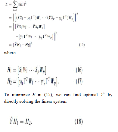 |
| The last embedding can be expressed by |
 |
| where H†1= HT 1 (H1HT 1 )−1 is the Moore–Penrose pseudoinverse of H1. Put YL and Yˆ together, we get embedding of all data points Y . |
| D. Proposed Algorithm and Approximate Analytic Projection |
| The main computation steps of LCA-GP can be summarized as follows. |
| 1) Find a set of TPLs, XL , by Algorithm 1. |
| 2) Apply global TCIE on XL and obtain the embedding YL in Rd . |
| 3) Construct the overlapping patches set based on the landmarks by (4) |
| 4) Obtain the local tangent coordinates of each patch Xi by (7) and compute Wi by (13). |
| 5) Compute H1 in (16) and H2 in (17) and obtain the embedding Yˆ by (19). |
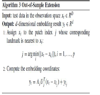
| 6) Put YL and Yˆ together to get the last embedding Y . In the first step, computing LM and updating it involves calculating shortest paths from p TPLs to other nodes on the graph. With Fibonacci heap, these take O(pNlogN). Computing LE and updating it take O(pN). As to run TCIE, since the geodesic distances between TPLs has been calculated in the previous step, solving the MDS optimization problem takes O(p2D) and the boundary detection takes O(p2). Calculating the local coordinates of all patches takes O(NDmin(2N/p, D)). The fifth step is to solve a linear system with the computational complexity O(N3) and for alarge dataset it consumes most of the time.Like almost all other methods for nonlinear dimensionality reduction, LCA-GP provides an embedding of a train set of data points. Often, we need to project a test data point that is outside the train set. The problem is an “out-ofsample extension” [39]. In our algorithm, each data point belongs to two patches, patch i and patch j. We have |
 |
| where ei and e j are error terms and are very small. If the error term is ignored, then we approximately find transformation from each local linear model to the global coordinate space as follows: |
 |
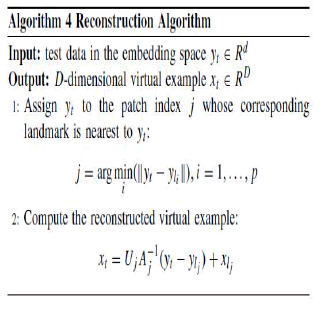
| The mapping function gives an explicit forward mapping from the observation space to the embedding space. Furthermore, its reverse mapping can be easily deduced in an entirely inverse manner |
 |
| Once the mapping function between the two spaces is built through a mixture of linear transformations, when applying to new test data, LCA-GP only needs first to identify to which patch the test data belongs and then to perform the corresponding transformation. Specifically, Algorithms 3 and 4 are designed to generalize the train results to unseen cases in the observation and embedding space, respectively. As a result, the train set is no longer required for subsequent process, leading to significant computational and storage savings. |
 |
 |
| E. Comparisons With Previous Work It can be seen that LCA-GP bears some resemblance to LTSA and subsequent methods [30], [34]. Generally speaking, these methods all share the (similar) philosophy of aligning local coordinates in a global coordinate space. However, there are some significant differences between LCA-GP and the other methods. First, the constituted finite |
| open covers of the manifold by these methods are different from each other. Second, LCA-GP solves the problem of optimum alignment differently from other methods. Progressive alignment method used in [34] and [35] is absolutely different from the proposed one. It aligns local coordinates patch by patch. Both LCAGP and the one in [18] and [30] try to minimize the global alignment error; however, as to minimize objective function, due to the introduction of landmarks, our LA algorithm is quite different from others which we call conventional alignment (CA). CA first translates each patch such that the local coordinate (which equals to zero) of the mean point of the patch meets its global coordinate (which is unknown), and then rotates and scales all patches to minimize the global alignment error as follows: |
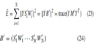 |
| and M_ = B_B_T . Consider that the problem to minimize (23) is ill-posed, and a constraint, i.e., YYT = I , is imposed to remove arbitrary translation and scaling. The LA method does not need to do so, and it first translates each patch such that the corresponding landmark’s local coordinate (which equals to zero) meets its global coordinate (which is known), and then rotates and scales all patches to minimize the global alignment error as in (15) which can be translated into a linear system in (18) without any constraints. LCA-GP has properties similar to those of FusionGL [23]. First, both LCA-GP and FusionGL use landmarks to preserve the global structure of manifold. Second, they fill the local models into the global coordinate space. We compare LCA-GP and FusionGL on these two issues. First, the two methods to select landmarks are different. It has been described in Section II. And the visualized comparison |
| results are shown in Fig. 2. Second, FusionGL uses semisupervised manifold learning methods with inexact inputs, i.e., it minimizes an objective function that combines the mapping error of landmarks with a regularization term. Sun et al. use SS-LLE and mention that SS-LTSA can be used as well. We first compare LA with SS-LTSA. From alignment standpoint, SS-LTSA is same as LTSA on the first two steps, i.e., the neighborhood of each data point constitutes one patch and PCA is used to derive local coordinates of all patches. As to the third step, SS-LTSA translates each patch such that the local coordinate of the mean point of the patch meets its global coordinate, and then rotates and scales all patches such that the local coordinates of the landmarks meet their global coordinates, while the global alignment error is minimized, i.e., adds a constraint on (23). Then |
 |
| where SL is a selection matrix such that XL = XSL. From the semisupervised manifold learning standpoint, (15) in LA can be reformulated as follows: |
 |
| where Si and Wi , i = 1,. . . . p, have the similar meaning of (14), Ri is 0–1 data selection matrix such that Y Ri = yli_T |
| and M = BBT . Partitioning Y and M, minimization of (26) becomes |
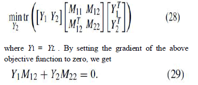 |
| We see that the global low-dimensional coordinates can be computed by solving a linear system of equations. Obviously, M in (26) is different from M_ in (25). For inexact landmarks information, FusionGL in fact minimizes an objective function that combines the mapping error with a regularization term as follows |
 |
| where Y ∗ 1 = YL , β is the regularization parameter that reflects the confidence level in landmarks information. In this way, the global coordinates of ladmarks can be optimized, but an approximate mapping function in closed form between highdimensional data space and low-dimensional embedding space cannot be derived and the out-of-sample problem will not be settled |
EXPERIMENTS |
| In this section, we systematically compare our method with other dimensionality reduction algorithms on both synthetic and real-world data. All algorithms are straightforwardly implemented in MATLAB. In most experiments, our algorithm is compared with six different dimensionality-reduction algorithms based on manifold learning, i.e., Isomap [8], LLE [11], LTSA [18], LMDS [30], LLI [34], and FusionGL [23]. In these algorithms, Isomap, LLE, and LTSA are three wellknown algorithms for nonlinear dimensionality reduction and LMDS and LLI are two representative alignmentbased algorithms devised recently. FusionGL is an algorithm similar to ours. |
 |
| A. Visualization Experiments |
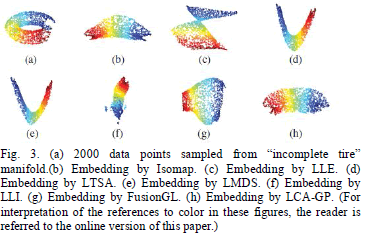
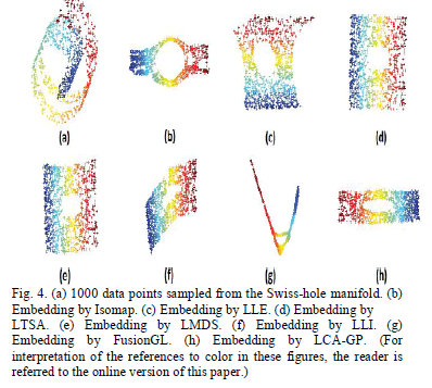
| In order to test the effectiveness of LCA-GP in visualized way, two synthetic datasets, which are more difficult to learn than some widely used datasets such as Swissroll and Scurve, and one image dataset are first employed. The manifold of “incomplete tire” cannot isometrically map to a lower dimensional Euclidean space and the manifold of “Swissroll with a hole” (Swiss-hole) is nonconvex. The Frey face images dataset is also used in [11] and [30]. The corresponding 2-D embedding results are shown in Figs. 3–5, respectively. The first dataset contains 2000 data points evenly sampled from an “incomplete tire” and is plotted in Fig. 3(a). Seven algorithms run on all data points and the parameters of each algorithm are selected carefully as follows. The neighbor parameter k in Isomap, LLE, and LTSA is 6, 12, and 8, respectively. The number of centers in LLI is 150. In LMDS and FusionGL, the neighbor parameter k is 8 and the overlapping factor α is 0.5. The other three parameters of FusionGL are selected using the method in [23], specifically, tl = 0.127, tg =∞, β = 10−4. In LCA-GP, the proportion of initial landmarks parameter α is 0.05, the neighborhood size to estimate the tangent space of alternative landmarks is 6, and the local linearity parameter η is 0.985. One important future work is to develop an adaptive algorithm to automatically tune the parameter η by relying on some kind of performance evaluation criterion [40]. The embedding result of Isomap contains many holes and distortion of shape [see Fig. 3(b)]. This is because Isomap cannot derive local structure well due to the inaccuracy of the computed geodesic distance matrix, and the mechanism of keeping the distances is only effective for globally iso neighborhood relations in the landmarks are wrong due to the existence of the hole and seriously distorted embedding of landmarks is derived by DPE based on these neighborhood relations. Our method [see Fig. 4(h)] finds of the manifold. This is due to the local isometric and global preserving properties of LCA-GP. |
 |
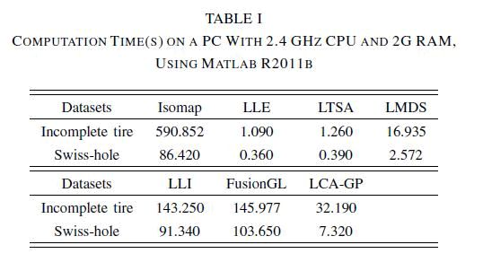 |
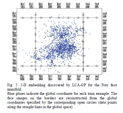
| In Section III-D, the computational complexity of LCAGP is analyzed by Big O. To further compare with the other algorithms, Table I reports the computation time of the experiments above. We see that LCA-GP is much faster than Isomap, LLI, and FusionGL, but slower than LLE, LTSA, and LMDS. Face recognition has been one of the most popular research topics in pattern recognition during this decade [41], [42]. A critical part in face recognition is the dimension reduction algorithm for feature extraction. We applied LCA-GP to the Frey face images dataset1 that has been used in [11] and [30]. The dataset consists of 1965 photographs taken of the same person with different poses and various facial expressions. Each photograph is a 20 × 28 grayscale image and therefore can be treated as a vector with 560 elements corresponding to raw pixel values, giving rise to inputs with D = 560 dimensions. Although the input dimensionality is quite high, the perceptually meaningful structure of these images is parameterized by fewer independent degrees of freedom pose and expression variables. We choose α = 0.05 |
| k = 16, and η = 0.6 empirically. Fig. 5 illustrates the 2- D embedding and some reconstructions. Similar to previous work [30], the 2-D embedding correctly discovers the two dominant variations in the face manifold, one for pose and another for expression. One may also see that some reconstructions, especially those near the boundary, are not good enough. This is mainly because the reconstruction algorithm is one kind of approximate algorithm, and, further, the model is extrapolating from the train images to low sample density regions. |
 |
| B. Data Clustering |
| We apply the proposed and existing manifold learning algorithms to two handwritten digits databases, i.e., the USPS dataset2 and the MNIST dataset,3 and then perform Kmeans clustering to compare the results of different algorithms in these tests. The USPS dataset contains 1100 grayscale images of each of the 10 digits from “0” to “9.” Each image is sized as 16 × 16 and converted to D = 256 dimensional vector. The MNIST dataset has a training set of 60 000 images and a testing set of 10 000 images. In our experiments, we take the first 1000 images from training set and the first 1000 images from testing set as our dataset. Each digit contains around 200 images. Each digit image is of size 28 × 28 and therefore represented by a D = 784 dimensional vector. The clustering algorithm generates a cluster label for each data point. The clustering performance is evaluated by comparing the generated class label and the ground truth. In our experiment, accuracy is used to measure the clustering performance. Given a point xi, let ri and si be the obtained cluster label and the label provided by the ground truth, respectively. The accuracy is defined as follows: |
 |
 |
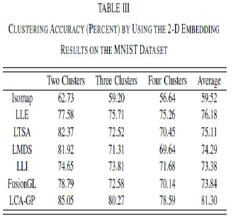 |
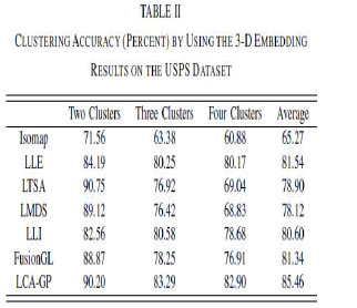
| where N is the total number of data points and δ(x, y) is the delta function which is equal to 1 if x = y and 0 otherwise, and map(ri ) is the permutation mapping function that maps each cluster label ri to the equivalent label from the dataset. The best mapping can be found by using the Kuhn–Munkres algorithm. The evaluations are conducted by using different numbers of clusters (K), i.e., K = 2, 3, 4. For each given cluster number K, 10 test runs are conducted on a subset of the data made of samples from K randomly chosen classes, and the final performance scores are computed by averaging the scores from the 10 tests. All algorithms are evaluated on the same combinations of K classes. We apply different algorithms to 3-D embedding (USPS) or 2-D embedding (MNIST) and apply K-means for clustering. The Kmeans is applied 10 times with different start points, and the best result in terms of the objective function of Kmeans is recorded. Table II shows the clustering accuracy by using 3-D embedding for each algorithm on the USPS dataset, and Table III shows the clustering accuracy by using 2-D embedding for each algorithm on the MNIST dataset. As can been seen, LCA-GP outperform the other six algorithms. In Table II, LTSA achieves 90.75% clustering accuracy while our method achieves 90.2% when the number of clusters is 2, but the average accuracy of LTSA is lower than ours. This is because the imposed unit covariance constraint of LTSA results in the deficiency of global metrics and undesired rescaling of the manifold, which may impact the clustering results, and the more the number of clusters, the larger the impact. |
| C. Pose Estimation |
| In this subsection, we use the oriental face database4 for head pose estimation to test the performance of LCA-GP. |
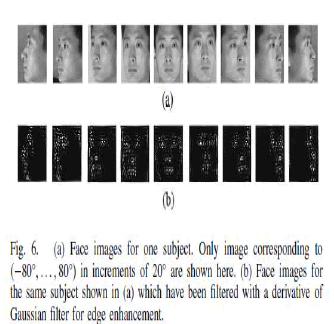 |
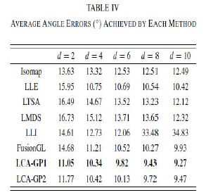
| The database consists of 33 669 images of 1247 people in JPEG format. We extract a typical subset of the oriental face database, which contains face images of 20 different individuals; each individual has 19 face images with pose angle views varying from −90° to 90° in increments of 10°. The face samples are prepared in the following manner. First, face-only images are automatically extracted from the original images and further subjected to the following preprocessing: grayscale images are formed [see Fig. 6(a) for an example], which are subsequently transformed to edge images by using a derivative of Gaussian filter [see Fig. 6(b) for an example]. The resulting images are scaled to a constant size (20 × 21 pixels) and stored as 420-D vectors to be used as training/testing samples. Because the objective of the first experiment is to compare the performance of different manifold learning algorithms and most of the six algorithms listed at the beginning of Section IV do not address out-of sample extensions, we adopt the following experimental procedure: we run each of the seven methods (including ours) on all the 380 samples which includes 200 training samples and 180 testing samples to derive the d-dimensional embedding of test samples and use a linear method proposed in [43] to obtain their view angles. Specifically, let X be all samples, Xtn be the train samples, and Xt t be the test samples. For each manifold learning method, we first derive the d-dimensional embedding of Xtn, Ytn, and a linear pose parameter map F is calculated from tn = FYtn, where tn is a matrix of the view angles of the training samples. Then the embedding of Xt t , Yt t is derived by running the corresponding manifold method on X. The resulting viewangles of the test samples can be estimated by t t = FYt t . Table IV illustrates the average angle errors obtained by each algorithm, as d is set to 2, 4, 6, 8, and 10, respectively. |
| The row corresponding to LCA-GP1 is the results of our method by the above procedure. As can be seen from Table IV, the proposed LCA-GP-based procedure finds more significant embedding space than the other six methods and achieves the lowest estimation errors. This may be due to the TPLs which can effectively guarantee the linear property in each local patch and to the LA method which can preserve the manifold structure better. To verify the effectiveness of out-of-sample extension of LCA-GP, we modify some steps of the above procedure. Specifically, Yt t is derived by running out-of-sample extension of LCA-GP. The row corresponding to LCAGP2 in Table II shows the average angle errors obtained in this way. It can be seen that, in all cases, the difference between LCA-GP1 and LCA-GP2 is very small. This indicates that the derived approximate analytic projections between the observation space and the embedding space are useful in real applications. |
 |
CONCLUSION |
| In this paper, we described a novel alignment-based manifold learning method. Compared with the classic Isomap and LLE, our algorithm can well preserve both the local geometry and global structure of the manifold. In comparison with the existing alignment-based methods such as LTSA and LMDS, LCA-GP derives more reasonable and efficient local models, and preserves the relationships between patches in original space during the alignment process without the unit covariance constraint. Compared with the related twostep method such as FusionGL, LCA-GP finds the TPLs which can reflect the structure of manifold better, and further approximately derives a parametric function for out-of-sample extension. Experimental results on both synthetic data and image datasets in Section IV indicate that LCA-GP obtains better embedding. Even so, still there are some problems that remain. For one thing, instead of empirical selection, developing an adaptive algorithm to automatically tune the parameter η in LCA-GP is a challenging and interesting task. Moreover, because of TCIE’s failure for those manifolds that cannot be isometrically mapped to a lower dimensional Euclidean space, developing a more effective method to derive the global coordinates of landmarks may also be an important direction in future works. In addition, inspired by FusionGL, we propose to investigate a more flexible algorithm to optimize the global coordinates of landmarks in the LA step. |
References |
|