International Journal of Innovative Research in Science, Engineering and Technology
ISSN ONLINE(2319-8753)PRINT(2347-6710)
ISSN ONLINE(2319-8753)PRINT(2347-6710)
Sweta K. Shah1, Prof. D.U. Shah2
|
| Related article at Pubmed, Scholar Google |
Visit for more related articles at International Journal of Innovative Research in Science, Engineering and Technology
Image Fusion is the process in which two or more images are combined into single image which can retain all important features of all original image. Fused image will be more informative and complete than any of the input images. This paper presents two approaches to image fusion, namely Spatial Fusion and Transform Fusion . This paper describes Techniques such as Principal Component Analysis which is spatial domain technique and Discrete Wavelet Transform , Stationary Wavelet Transform which are Transform domain techniques. Performance metrics without reference image are implemented to evaluate the performance of image fusion algorithm. Experimental results shows that image fusion method based on Stationary Wavelet Transform is remarkably better than Principal Component Analysis and Discrete Wavelet Transform.
Keywords |
| Image Fusion, Principal Component Analysis, Discrete Wavelet Transform, Stationary Wavelet Transform. |
INTRODUCTION |
| Fusion is a process which can be used to improve quality of information from a set of images . By the process of image fusion the good information from each of the given images is fused together to form resultant image whose quality is superior to any of input images. There are important requirements for image fusion process[6]: |
| -The fused image should preserve all relevant information from the input images. |
| -Image fusion should not introduce artifacts which can lead to wrong diagnosis. |
| In the field of remote sensing, medical imaging and machine vision the multi-sensor data may have multiple images of the same scene providing different information. As optical lenses in charged coupled devices have limited depth of focus, it is not possible to have a single image that contains all the information of objects in the image, so image fusion is required. |
| There are two groups into which image fusion methods are divided, namely Spatial domain fusion method and Transform domain fusion method. Spatial domain fusion method will directly deal with pixels of input images. In Transform domain fusion method image is first transformed into frequency domain. |
RELATED WORK |
| During the past two decades, many image fusion methods are developed. According to the stage at which image information is integrated, image fusion algorithms can be categorized into pixel, feature, and decision levels. The pixellevel fusion integrates visual information contained in source images into a single fused image based on the original pixel information. In the past decades, pixel-level image fusion has attracted a great deal of research attention. Generally, these algorithms can be categorized into spatial domain fusion and transform domain fusion. The spatial domain techniques fuse source images using local spatial features, such as gradient, spatial frequency, and local standard derivation. For the transform domain methods, source images are projected onto localized bases which are usually designed to represent the sharpness and edges of an image. Therefore, the transformed coefficients (each corresponds to a transform basis) of an image are meaningful in detecting salient features. Consequently, according to the information provided by transformed coefficients, one can select the required information provided from the source images to construct the fused image[9]. |
| Zhang and Blum established a categorization of multiscale decomposition-based image fusion to achieve a high-quality digital camera image[12]. They focused mainly on fusing the multiscale decomposition coefficients. For this reason, only a few basic types were considered, i.e. the Laplacian pyramid transform, the DWT, and the discrete wavelet frame (DWF). Only visible images were considered in performance comparisons for digital camera application. Pajares and Cruz gave a tutorial of the wavelet-based image fusion methods[14]. They presented a comprehensive comparison of different pyramid merging methods, different resolution levels, and different wavelet families. Three fusion examples were provided, namely multi-focus images, multispectral-panchromatic remote sensing images, and functional– anatomical medical images[9]. |
| Image fusion methods based on Multiscale Transforms (MST) are a popular choice in recent research. MST fusion uses Pyramid Transform (PT) or Discrete Wavelet Transform (DWT) for representing the source image at multi scale. DWT approach is considered and it uses area level maximum selection rule and a consistency verification step. But, DWT suffers from lack of shift invariance and poor directionality. But, the un-decimated DWT, namely Stationary Wavelet Transform (SWT) is shift invariant and Wavelet Packet Transform (WPT) provides more directionality. This benefit comes from the ability of the WPT to better represent high frequency content and high frequency oscillating signals in particular. The Multi Wavelet Transform (MWT) of image signals produces a nonredundant image representation, which provides better spatial and spectral localization of image formation than DWT[7]. |
SPATIAL DOMAIN TECHNIQUE |
A. Principal Component Analysis |
| Principal component analysis (PCA) is a vector space transform often used to reduce multidimensional data sets to lower dimensions for analysis. PCA is the simplest and most useful of the true eigenvector-based multivariate analyses, because its operation is to reveal the internal structure of data in an unbiased way. If a multivariate dataset is visualized as a set of coordinates in a high-dimensional data space (1 axis per variable), PCA supplies the user with a 2D picture, a shadow of this object when viewed from its most informative viewpoint. This dimensionally-reduced image of the data is the ordination diagram of the 1st two principal axes of the data, which when combined with metadata (such as gender, location etc) can rapidly reveal the main factors underlying the structure of data[1]. |
| Basically Principal component analysis is a technique in which number of correlated variables are transformed into number of uncorrelated variables called principal components. A compact and optimal description of datasets is computed by PCA. The first principal component accounts for as much of the variance in the data as possible and each succeeding component accounts for as much of the remaining variance as possible. First principal component is taken to be along the direction with maximum variance. The second principal component is constrained to lie in the subspace perpendicular to the first within this subspace, this component points the direction of maximum variance. The third principal component is taken in the direction of maximum variance in the subspace perpendicular to the first two and so on. The PCA is also called as Karhunen-Loève transform or the Hotelling transform. The PCA does not have a fixed set of basis vectors like FFT, DCT and wavelet etc. and its basis vectors depend on the data set [2]. |
| Let X be a d-dimensional random vector and assume it to have zero empirical mean. Orthonormal projection matrix V would be such that Y =VT X with the following constraints. The covariance of Y, i.e., cov(Y) is a diagonal and inverse of V is equivalent to its transpose ( V−1= VT). Using matrix algebra |
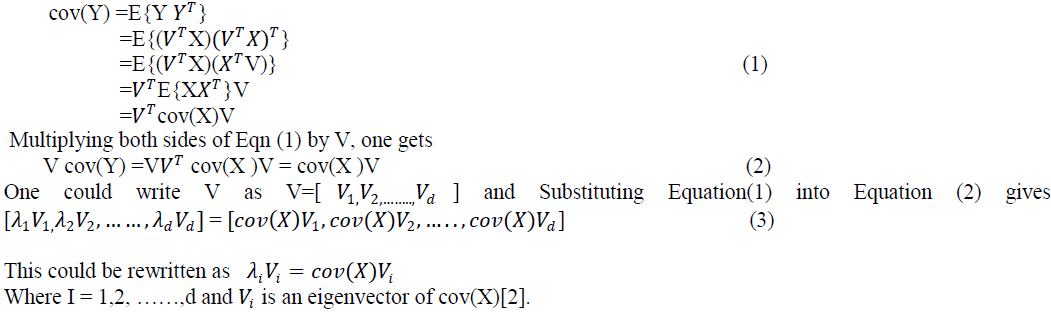 |
| Image fusion process using PCA is described below : |
| The information flow diagram of PCA-based image fusion algorithm is shown in Fig.1 . |
| ïÿýïÿý1 (x, y) and ïÿýïÿý2 (x, y) are the two input images which are to be fused[2]. |
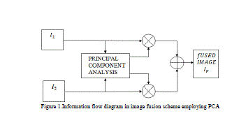 |
| -From the input image matrices produce the column vectors. |
| -Compute the covariance matrix of two column vectors formed before. |
| -Compute the Eigen values and Eigen vectors of the covariance matrix. |
| The column vector corresponding to the larger Eigen value is normalized by dividing each element with mean of Eigen vector. |
| Normalized Eigen vector value act as the weight values which are respectively multiplied with each pixel of the input images. |
| -The fused image matrix will be sum of the two scaled matrices . |
TRANSFORM DOMAIN TECHNIQUES |
A. Discrete Wavelet Transform |
| Wavelet theory is an extension of Fourier theory in many aspects and it is introduced as an alternative to the short-time Fourier transform (STFT). In Fourier theory, the signal is decomposed into sines and cosines but in wavelets the signal is projected on a set of wavelet functions. Fourier transform would provide good resolution in frequency domain and wavelet would provide good resolution in both time and frequency domains. Although the wavelet theory was introduced as a mathematical tool in 1980s, it has been extensively used in image processing that provides a multiresolution decomposition of an image in a biorthogonal basis and results in a non-redundant image representation. The basis are called wavelets and these are functions generated by translation and dilation of mother wavelet. In Fourier analysis the signal is decomposed into sine waves of different frequencies. In wavelet analysis the signal is decomposed into scaled (dilated or expanded) and shifted (translated) versions of the chosen mother wavelet or function . A wavelet as its name implies is a small wave that grows and decays essentially in a limited time period. A wavelet to be a small wave, it has to satisfy two basic properties[2]: |
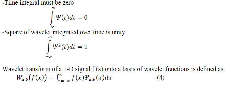 |
| Basis is obtained by translation and dilation of the mother wavelet as: |
| The mother wavelet would localise in both spatial and frequency domain and it has to satisfy zero mean constraint. In discrete wavelet transform (DWT), the dilation factor is a=2 and the translation factor is b= n2 , where m and n are integers. |
| In discrete wavelet transform (DWT) decomposition, the filters are specially designed so that successive layers of the pyramid only include details which are not already available at the preceding levels. |
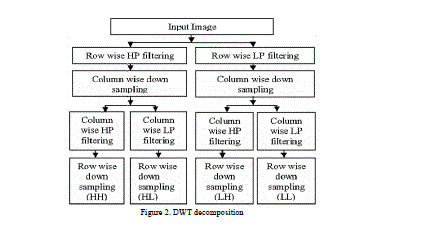 |
| The DWT decomposition[3] uses a cascade of special lowpass and high-pass filters and a sub-sampling operation. The outputs from 2D-DWT are four images having size equal to half the size of the original image. So from first input image we will get HHa, HLa, LHa, LLa images and from second input image we will get HHb, HLb, LHb, LLb images. LH means that low-pass filter is applied along x and followed by high pass filter along y. The LL image contains the approximation coefficients. LH image contains the horizontal detail coefficients. HL image contains the vertical detail coefficients, HH contains the diagonal detail coefficients. The wavelet transform can be performed for multiple levels. The next level of decomposition is performed using only the LL image. The result is four sub-images each of size equal to half the LL image size. |
| Image fusion process using DWT is described below: |
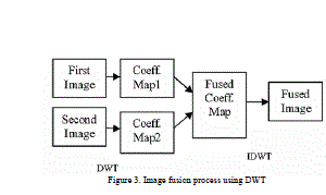 |
| Wavelet transform is first performed on each source images to generate a fusion decision map based on a set of fusion rules. The fused wavelet coefficient map can be constructed from the wavelet coefficients of the source images according to the fusion decision map. Finally the fused image is obtained by performing the inverse wavelet transform. The process steps can be given below[3]: |
| -Accept the two images. |
| -Perform DWT on both images A and B. |
| -Perform level 2 DWT on both images A and B |
| -Let the DWT coefficient of image A will be [HHa HLa LHa LLa]. |
| -Let the DWT coefficient of image B will be [HHb HLb LHb LLb] |
| -Take the average of pixels of the two band from HHa and HHb and store to HHn. |
| `-Take the average of pixels of the two band from HLa and HLb and store to HLn. |
| -Take the average of pixels of the two band from LHa and LHb and store to LHn. |
| -Take the average of pixels of the two band from LLa and LLb and store to LLn. |
| -Now we have new HHn, HLn, LHn, LLn DWT coefficients. |
| -Take Inverse DWT on the HHn, HLn, LHn, LLn coefficients. |
| -Obtain the fused image and display. |
B. Stationary Wavelet Transform |
| The Discrete Wavelet Transform is not a time invariant transform. The way to restore the translation invariance is to average some slightly different DWT, called un-decimated DWT, to define the stationary wavelet transform (SWT). It does so by suppressing the down-sampling step of the decimated algorithm and instead up-sampling the filters by inserting zeros between the filter coefficients. Algorithms in which the filter is upsampled are called “à trous”, meaning “with holes”. As with the decimated algorithm, the filters are applied first to the rows and then to the columns. In this case, however, although the four images produced (one approximation and three detail images) are at half the resolution of the original; they are the same size as the original image. The approximation images from the undecimated algorithm are therefore represented as levels in a parallelepiped, with the spatial resolution becoming coarser at each higher level and the size remaining the same. Stationary Wavelet Transform (SWT) is similar to Discrete Wavelet Transform (DWT) but the only process of down-sampling is suppressed that means the SWT is translation-invariant. The 2-D SWT decomposition scheme is illustrated in Figure 4. |
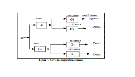 |
| The 2D Stationary Wavelet Transform (SWT) is based on the idea of no decimation. It applies the Discrete Wavelet Transform (DWT) and omits both down-sampling in the forward and up-sampling in the inverse transform. More precisely, it applies the transform at each point of the image and saves the detail coefficients and uses the low frequency information at each level. The Stationary Wavelet Transform decomposition scheme is illustrated in Figure 4 where Gi and Hi are a source image, low pass filter and high-pass filter, respectively. Figure 4 shows the detail results after applying SWT to an image using SWT at 1 to 4 levels[7]. |
| Image fusion process using SWT is described below: |
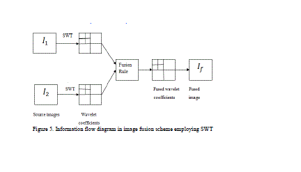 |
| The information flow diagram of SWT-based image fusion algorithm is shown in Fig.5 |
| ïÿýïÿý1 (x, y) and ïÿýïÿý2 (x, y) are the two input images which are to be fused. In SWT scheme, the source images ïÿýïÿý1 (x, y) and ïÿýïÿý2 (x, y), are decomposed into approximation and detailed coefficients at required level using SWT. The approximation and detailed coefficients of both images are combined using fusion rule . The fused image could be obtained by taking the inverse Stationary wavelet transform. The process flow can be given below[7]: |
| The two source images are decomposed using SWT at one level resulting in three detail subbands and one approximation subband (HL, LH, HH and LL bands). |
| - Then average of approximate parts of images is taken. |
| The absolute values of horizontal details of image is taken and from the first part of image second part is subtracted. D=(abs(H1L2)-abs(H2L2))>=0 |
| -Make element wise multiplication of D and horizontal detail of first image for fused horizontal part and then subtract another horizontal detail of second image multiplied by logical not of D from first. |
| -Find D for vertical and diagonal parts and obtain fused vertical and diagonal detail of image. |
| -Repeat same process for fusion al first level. |
FUSION PARAMETERS |
| Image Quality is a characteristic of an image that measures the perceived image degradation. Imaging systems may introduce some amounts of distortion or artifacts in the signal, so the quality assessment is an important problem. There are several techniques and metrics that can be measured objectively and automatically evaluated by a computer program. Therefore, they can be classified as Full Reference Methods (FR) and No-Reference Methods (NR). In FR image quality assessment methods, the quality of a test image is evaluated by comparing it with a reference image that is assumed to have perfect quality. NR metrics try to assess the quality of an image without any reference to the original one. Image quality and metrics considered and implemented here fall in the NR category[8]. |
| Fusion performance can be measured by the following fusion quality evaluation metrics’: |
A. Spatial Frequency(SF): |
| Spatial Frequency indicates the overall activity in the fused image. The SF is computed as[2]: |
| Row Frequency: |
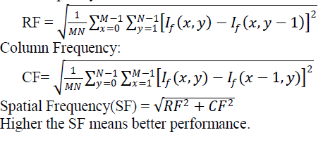 |
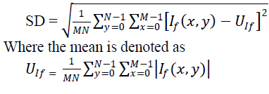
B. Standard Deviation(SD): |
| Standard Deviation measures the contrast in the fused image. Fused image with high contrast would have high standard deviation[2]. |
 |
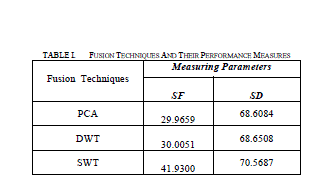
RESULTS |
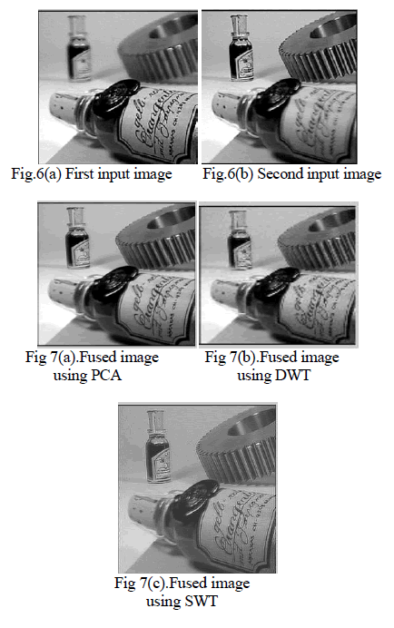 |
 |
CONCLUSION |
| In this paper image fusion using spatial domain and transform domain techniques is implemented. In spatial domain principal component analysis is implemented and in transform domain discrete wavelet transform and stationary wavelet transform are implemented. Spatial domain method have blurring problem. The transform domain methods provide a high quality spectral content. But DWT in transform domain is time invariant, this problem is overcome by using SWT . It can be concluded from SF and SD values that SWT is better image fusion technique compared to PCA and DWT. |
References |
|