ISSN ONLINE(2319-8753)PRINT(2347-6710)
ISSN ONLINE(2319-8753)PRINT(2347-6710)
| D. R. Prajapati Assistant Professor, Department of Mechanical Engineering, PEC University of Technology (formerly Punjab Engineering College), Chandigarh, India |
| Related article at Pubmed, Scholar Google |
Visit for more related articles at International Journal of Innovative Research in Science, Engineering and Technology
Control charts have been used to monitor and control the production process and generate some sort of signal when there are indications to the effect that the process has gone out of control. Conventional (Shewhart) X charts were originally developed by Walter F. Shewhart (1931). The limits of the chart are known as upper control limit (UCL) and lower control limit (LCL). He suggested two control limits i.e. UCL = X + 3σ/√n and LCL = X - 3σ/√n, where X is the target mean, σ is population standard deviation and n is the sample size. In implementing the X chart, it is assumed that the process outputs must be IID but usually there is some correlation among the data. When this correlation builds up automatically in the entire process, this phenomenon is called autocorrelation. It is found that the performance of conventional X chart deteriorates on increasing the level of correlation.
Keywords |
| Average run length, sample size, X charts, IID data and Autocorrelation |
INTRODUCTION |
| The process is assumed to be out of control when the sample average falls beyond these limits. The Shewhart X chart is more useful to detect large shifts (> 2σ) in process mean. Several researchers examined the performance of control charts in the presence of autocorrelation. If process measurements are autocorrelated, then standard constructions of control charts will violate the assumption that samples are independent. The Type-I error rate for control charts is sensitive to autocorrelated data i.e. control charts are subjected to increased false alarms. Even at low levels of correlation, dramatic disturbances can occur in the chart properties |
A. Classification of Control charts |
| Basically, control charts can be classified as: (i) Control charts for variables and (ii) Control charts for attributesThe control charts for variables are used for quality characteristics which are measurable like length, diameter, tensile strength, temperature, viscosity etc. while the control charts for attributes are used for quality characteristics which are non-measurable. Control charts for variables may further be classified as:ïÃâ÷ Control charts for monitoring the process means (averages) ïÃâ÷ Control charts for monitoring the process dispersion ïÃâ÷ Combined control charts ïÃâ÷ Control charts for monitoring autocorrelated dataThe process is assumed to be out of control when the sample average falls beyond these limits. If a variable has a normal distribution with mean of zero and standard deviation of one, and a X chart is used with control limits at ±3σ, the ARL will depend upon the sample size. ARLs for sample size of four are given in Table 1.A quality engineer may like his chart to generate a signal when the process average shifts by an amount equal to the process standard deviation. However an ARL of 44 may be too high as, on the average, the process will operate in an uncontrolled manner for a long period of time till 44 samples are inspected. |
A. Autocorrelation |
| In general, it is assumed that the process outputs must be IID but usually there is some correlation among the data. When this correlation builds up automatically in the entire process, this phenomenon is called autocorrelation. The observations from the process output are usually positively correlated in most of the cases. In this case, if the current observation is on one side of the mean, the next observation will most likely be found on the same side of the mean. Positively correlated data are characterized by runs above and below the mean. Positive correlation is more often encountered in practice than negative autocorrelation. When X charts are applied to the autocorrelated data, the false alarm rate increases and performance of the X chart is suspected. So improvement in the (Shewhart) X chart is needed to improve its performance for the correlated data. The following section deals with the literature review in this area. Various researchers contributed in detecting the autocorrelation in data and modified the X charts. For the simulation of data, Markov chain, Monte Carlo, Time– series approach, MATLAB are widely used by the researchers. The research work done so far in modifying the X chart for the autocorrelated data is discussed as follows: Kramer and Schmid (2000) discussed the behavior of the Shewhart residual chart and the modified Shewhart chart for unknown parameters of the underlying process. They focused on the estimation of the variance. For autoregressive models (AR models), they considered the estimation of the AR coefficients. They finally compared the ARL of the control chart with estimated parameters with the ARL of the scheme for known parameters and with the ARL for independent variables. Chiu and Yang (2001) suggested that neural networks can be used to identify shifts in correlated process parameters. They developed and trained the back propagation neural networks to identify shifts in process parameter values. They used all-possible-regression selection procedures for finding the appropriate numbers of input nodes to use in a neural network model. They found that the neural networks are successful at identifying shifts at one, one and half, and two standard deviations from the target. They concluded that the neural networks outperform the traditional SPC approaches in identifying shifts in process parameters. |
| Noorossana et al. (2003) presented an artificial neural network (ANN) model for detecting and classifying three types of non-random disturbances referred to as level shift, additive outlier and innovational outlier, which are common in autocorrelated processes. An autoregressive model of order one, AR(1) model was considered to characterize the quality characteristic of interest in a continuous process where autocorrelated observations were generated over time. The performance of the proposed procedure was evaluated through the use of a numerical example. Preliminary results indicated that the procedure could be used effectively to detect and classify unusual shocks in autocorrelated processes. Castagliola and Tsung (2005) investigated the effect of skewness on conventional autocorrelated SPC techniques and provided an effective approach based on a scaled weighted variance approach to improve SPC performance in such an environment. Gauri and Chakraborty (2008) used artificial neural network (ANN) to recognize different control chart patterns (CCPs). ANN with features extracted from the process data as input vector representation could facilitate efficient pattern recognition with a smaller network size. A set of seven shape features were selected, whose magnitudes are independent of the process mean and standard deviation under a special representation of the sampling interval in the control chart plot. Chen and Cheng (2009) found that in the design of the X control chart, both the sample size, „mâÃâ¬ÃŸ of X and the control-limits factor, „kâÃâ¬ÃŸ (the number of standard deviations from the center line) must be determined. They analyzed under the assumption that the quality characteristic, follows an autocorrelated process with known covariance structure but unknown marginal distribution shape. |
| Prajapati and Mahapatra (2009) provided a survey and brief summary of the work on the control charts for variables to monitor the process mean and dispersion from 1931 to 2008. Kiran et al. (2010) carried out a study on training algorithms for control charts pattern recognition and selected the best two patterns with their optimal structure for both type I and type II errors for generalization without early stopping and with early stopping and proposed the best one. Wu and Yu (2010) proposed a neural network-based identification model for both mean and variance shifts in correlated processes. The proposed model uses a selective network ensemble approach named DPSOEN (Discrete Particle Swarm Optimization) to obtain the improved generalization performance, which outperforms those of single neural network. Costa and Castagliola (2011) found that measurement error and autocorrelation have an adverse effect on the performance of X chart. In order to counteract the undesired effect of autocorrelation, they built-up the samples with non-neighboring items, according to the time the items are produced. They also measured the quality characteristic of each item of the sample several times. The chart's performance was assessed when multiple measurements are applied and the samples are built by taking one item from the production line and skipping one, two or more before selecting the next. McCracken and Chakraborti (2013) presented an overview of the literature covering some of the one-and two-chart schemes, including those that are appropriate in parameters known (standards known) and unknown (standards unknown) situations. They also discussed some of the joint monitoring schemes for multivariate processes, autocorrelated data, and individual observations. In addition, they discussed some available nonparametric schemes for jointly monitoring location and scale and recommended some areas of further research. |
| The formulation of the autocorrelated numbers is discussed in the next section |
III. FORMULATION OF AUTOCORRELATED DATA |
| In the autocorrelated series of observation, each individual observation is dependent upon the previous observation. A series of positively autocorrelated numbers with a mean of zero and standard deviation of one is generated, using the MATLAB at various levels of correlation (Φ). Assuming N pairs of observations on two variables, x and y. The correlation coefficient between x and y is given by equation (1). Some authors use coefficient of correlation (Φ) instead of “r”. |
 |
| Where, the summations are over the N observations. The series generated are positively correlated in nature. For each level of correlation (Φ), various schemes of X chart are developed, using MATLAB. The detailed procedure to implement the X chart is explained in the following section. |
IV. PROCEDURE |
| The data are simulated with the help of MATLAB software. The autocorrelated numbers are generated from the series of data, taken from the standard normal distribution with mean of zero and standard deviation of one. The following procedure may be adopted to calculate the ARLs of the X chart. Values of width of control limits (L) are adjusted in such a way that they generate the in-control average run length (ARL) of approximately 370 in all the presented schemes for all the sample sizes is adopted to calculate The ARLs for sample size of ten at various levels of correlation are computed as per the given procedure.Step 1 Take the observations from industry at random basis. Step 2 Observations are generated randomly at a given mean and standard deviation. Step 3 For simulation, 10,000 observations with a sample sizes (n) of 10 are generated. Step 4 The observations are generated in such a way that there should be positive correlation with their previous data. Step 5 Those sets of parameters of the X chart, which give the in-control ARL Of approximately 370, are considered for comparison. Step 6 For the selected combinations, the ARLs are calculated at various shifts in process mean at different width of the control limits (L) and at the each levels of correlation (Φ). |
| Step 7 Optimal schemes of modified X chart are obtained for levels of correlation (Φ) of 0.00, 0.25, 0.50, 0.75 and 1.00. |
| Next section deals with the computation of ARLs of the X chart for sample size of 10 and at different levels of correlation (Φ). |
V. CONVENTIONAL X CHART FOR SAMPLE SIZE (N) OF TEN |
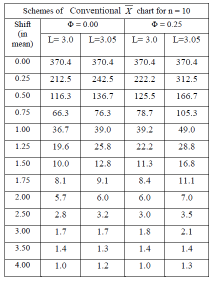
| Various schemes of the conventional X chart for sample size of ten are developed at various levels of correlation (Φ). Table 2 shows the various schemes of conventional X chart for sample size (n) of ten at the levels of correlation (Φ) of 0.00 and 0.25. Table 2 Schemes of Conventional X chart for sample size (n) of ten at Φ = 0.00 and 0.25 |
 |
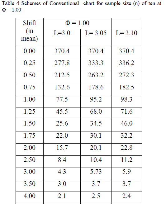
| Table 3 shows the various schemes of conventional X chart for sample size (n) of ten at the levels of correlation (Φ) of 0.50 and 0.75. Table 3 Schemes of Conventional X chart for sample size (n) of ten at Φ = 0.50 and 0. Table 4 shows the various schemes of Conventional X chart for sample size (n) of ten at the level of correlation (Φ) of 1.00. |
 |
| These schemes of the conventional X chart for sample sizes of 10 are analyzed at various levels of correlation (Φ). Analysis of these schemes is presented in the next section. |
VI. ANALYSIS |
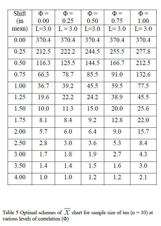
| Those schemes of conventional X chart which give quick response to the shift in the process mean are known as optimal schemes for a given sample size (n) and level of correlation (Φ). These schemes have the lower ARLs than others schemes for all the shifts. The performance of these schemes at the various shifts in the process mean and at different levels of correlation (Φ) is given in the Tables 5 |
 |
| i) The in-control Average run length (ARL) of approximately 370 is maintained for all the suggested schemes of the conventional X chart. |
| (ii) For a particular sample size, when autocorrelation in the observations increases, the false alarm rate also increases.(iii) The sensitivity of a chart to detect shift in the process mean depends upon the sample size. |
| (iv) The performance of conventional X chart deteriorates on increasing the level of correlation. |
| (v) At level of correlation (Φ) of 0.25 and for 1σ shift in process mean, the out of control ARL is 39.2 while it is 77.5 at Φ = 1.00. |
VII. CONCLUSIONS |
| The effect of autocorrelation on the sample size of ten for conventional (Shewhart) X chart for the correlated observations is studied. The performance of the X chart is measured in terms of the Average Run Lengths (ARLs). It is concluded that if faster detection in the process mean is desired, it is recommended to use larger sample sizes (n). The optimal schemes for sample size of 10 at different levels of the correlation have been suggested that may be very useful from the quality control point of view for many industries. This control chart may also be very useful for the service sectors also. |
References |
|