International Journal of Innovative Research in Science, Engineering and Technology
ISSN ONLINE(2319-8753)PRINT(2347-6710)
ISSN ONLINE(2319-8753)PRINT(2347-6710)
| Sanjib Kumar Hota Lecturer, Madhusudan Institute of Cooperative Management, Bhubaneswar, Orissa, India |
| Related article at Pubmed, Scholar Google |
Visit for more related articles at International Journal of Innovative Research in Science, Engineering and Technology
The analysis of the effect of methodological difference in estimating the technical efficiency of production function of various agricultural farms drawn from different agro-climatic zones of odisha is the main objective of the study. The Data envelopment Analysis (DEA) and Artificial neural networks (ANN), viz. Multilayer Perceptron (MLP) and Radial Basis function (RBF) networks have been used in the study. The statistical software like Banixia frontier Analyst-7 (for DEA), MATLAB-ANN tool box (for MLP) and Neuro Solutions-6.0 have been used for estimating the technical efficiency through these models. The sensitivity analysis based on the optimum result of the network worked out by RBF has also been tested. The paper has illustrated the optimization problem by considering rice(paddy) crop yield data as the output (Y) and total Cost of Bullock/ Machine labor-per acre (X1), cost of human labor per acre (X2), Cost of seeds per acre (X3), Fertilizer cost per acre (X4), total-Irrigation Cost (X5), Cost of pesticide (X6) and Credit per acre (X7) and Gross cropped area under rice (X8) as inputs. It has been observed that the neural network-based estimation of technical efficiency may lead to a significant result; with radial basis function networks (RBFN) outperforming the other estimation techniques considered for the study. It is hoped that, in future, research workers would start applying these advanced ANN models to optimization problems relating to agricultural productivity.
Keywords |
| Data Envelopment Analysis, Artificial Neural Network, Technical Efficiency |
INTRODUCTION |
| The level of efficiency of a farmer in his production process is difficult to assess unless one is sure of the prevailing conditions in which he operates. For instance, a farmer may not be allocating his resources optimally due to resource constraints or the prevailing uncertainty with regard to price/yield or perhaps due to the lack of ready access to resources. Under such circumstances, he cannot be termed inefficient merely because he does not operate at the point where profit is maximized; profit maximization may not be his final objective. On the other hand, a farmer may be using all the inputs in required quantities, but may not be realizing the potential output due to improper management. In such cases, a comparison of output in relation to the level of inputs used reveals the true picture of efficiency. This is referred to as ‘technical efficiency’ which is the maximum possible yield achievable with a given level of input used (Jayaram et al., 1992) . Technical efficiency can also be defined as the farm’s ability to obtain the maximum output from a given set of resources (Farrell, 1957). In other words technical efficiency of a farm can be defined as the ability and willingness of the farm to obtain the maximum possible output with a specified endowment of inputs (represented by a frontier production function), given the technology and environmental conditions surrounding the farm (Mythili G. et al., 2000). As pointed out by Little et al (1987) comparison of indexes of technical efficiency of individual enterprises provides information on the relative as well as absolute levels of total factor productivity. For this reason measurement as well as interpretation of the technical efficiency of the individual farms in the area under study is an important exercise to do (Banik Arindam, 1994). |
II. RELATED WORK [ LITERATURE SURVEY] |
| A number of empirical study have been undertaken to measure the technical efficiency by using cross-section data with the help of both parametric and non-parametric techniques. In this regard the deterministic and stochastic frontier approach were used very popularly (Farrell, 1957), (Aigner and Chu, 1986), (Timmer, 1971), (Aigner, et al, 1977), (Meeuen and Broeck, 1977). A number of comprehensive work has been undertaken in this context by considering also the panel data approach and measurement of technical efficiency using cost functions (Forsund et al, 1980), (Bauer, 1990), (Battese, 1992) (Greene, 1993), (Kaliranjan and Shand, 1994) and (Kumbhakar, et al, 1997). However, only a few studies (Kaliranjan, 1981,Tadesse and Krishnamoorthy, 1997,Kaliranjan and Shand, 1994; Mythil and Shanmugam, 2000) have been carried out to measure technical efficiency of rice production in India using the cross-section data. The present study uses the nonparametric technique of Data Envelopment Analysis (DEA) to measure the technical efficiency of the farms cultivating rice for three different villages with different agrarian conditions of Bargarh district of Orissa during the agricultural year 2007-08. |
| In empirical production function analysis our prior knowledge about the technology that relates inputs and outputs is many times quite weak. Taking into account this fact, the two common approaches for measuring efficiency, linear programming methods like data envelopment analysis (DEA) and econometric techniques like multiple regression and in particular stochastic frontier analysis (SFA), assume only a few restrictions when estimating production frontiers. Traditional assumptions for DEA models are the convexity of the set of feasible input/output combinations, variable returns to scale and strong disposability of inputs and outputs. On the other hand, SFA has been modeled through Cobb-Douglas specifications or even through more flexible transcendental logarithmic (translog) form where we include non-linear effects into a linear parametric model. |
| Evolving from neuro-biological insights, artificial neural networks (ANNs) is a relatively young field of research with a rapid expansion in both theory and applications. Neural networks have shown during last decade to be especially useful for mapping problems under noise and uncertainty, when enough data example are available and particularly when inputs and outputs are related in non-linear ways which cannot be easily described in advance in linear equations. |
| Multiple linear regression modeling is widely used to estimate linear relationship between response variable and predictors. Its limitation is that it assumes the underlying relation between response and predictor variables to be “linear”. In real life situation, this assumption is rarely satisfied. Also, if there are several predictors, it is quite impossible to have an idea of the underlying non-linear functional relationship between response and predictor variables. To handle such a situation, “Artificial neural networks” (ANNs) is used. Cheng and Titterington (1994) have reviewed the ANN methodology from a statistical perspective, while Warner and Misra (1996) have laid emphasis on the understanding of ANN as a statistical tool. A distinguishing feature of ANNs that makes them valuable and attractive for a statistical task is that, as opposed to traditional model-based methods, ANNs are data-driven self-adaptive methods in that there are a few a-priori assumptions about the models for problems under study. This modeling approach with ability to learn from experience is very useful in many practical problems since it is often easier to have data than to have good theoretical guesses about the underlying laws governing the systems from which data are generated. Zhang (2007) has discussed various pitfalls in the ANN modeling work, which must be avoided. Most widely used ANN is multilayered feed forward artificial neural network (MLFANN). |
| Guermat and Hadri(1999) carried out a Monte Carlo experiment with the purpose of analyze the effects of functional form misspecifications and the performance of neural networks versus translog models for approximating different theoretical production functions like Cobb-Douglas, translog, CES function and Generalized Leontief model. They concluded that the neural network specification is a good alternative to the most commonly used translog model for measuring efficiency. |
| Daniel S. Gonzalez and A.V.Castro (2001) carried out a study with an objective to test how non-linearity of production functions affect estimations of technical efficiency obtained by ordinary and corrected least square (OLS, COLS), data envelopment analysis with constant and variable returns to scale (DEAcrs, DEAvrs), stochastic frontier analysis (SFA) and by Multilayer Perceptron (MLP) neural networks with backpropagation and have suggested through their findings that MLP is a flexible tool to fit production functions and a possible alternative to traditional techniques under non-linear contexts. |
| D.Pokrajac, J.Milutinovic and Z. Obradovic (2005) carried out a study with an objective of maximizing a profit function using a neural-based decision support system and evaluating the applicability of the method on simulated precision agriculture data. On the basis of experimental results they have suggested that the neural based profit maximization techniques may lead to a significant profit increase; with radial-basis function (RBF) networks outperforming multilayer perceptrons (MLP). |
| Jianhua Chen,(2005) has made an attempt for the empirical applications of that neural network methods to model agricultural economic issues and found that neural network methods outperformed the traditional econometric models including Multiple Regression. |
| R.K.Singh and Prajneshu (2008) carried out a study on the application of a particular type of ANN viz. multilayered feed forward artificial neural network (MLFANN) trained by two types of learning algorithms, namely Gradient descent algorithm (GDA) and Conjugate Gradient descent algorithm (CGDA) in the field of agriculture (i.e modeling and forecasting of maize crop yield) and also found the superiority of MLFANN over MLR in addressing the objectives of their study. |
| E.T.Venkatesh and P.Thangaraj (2008) carried out a study on the application of Self organizing Map and Multi-Layer Perceptron Neural Network based Data Mining in the field of agriculture and found desired solution from the analysis (i.e. clustering and predicting desired output against the inputs). |
| Hossein Hakimpoor, Khairil Anuar Bin Arshad, et.al. (2011) have reviewed some of the selected works done in application of ANNs in management sciences and concluded that Artificial Neural Networks (ANNs) are one of the tools that have become a critical component of business intelligence. |
| Chusnul Arif, Masaru Mizoguchi et.al. (2012) have attempted to apply an Artificial Neural Networks (ANN) model to estimate soil moisture in paddy field under different weather conditions between the two paddy cultivation periods and found that the ANN model reliably estimates soil moisture with limited meteorological data. |
III. OBJECTIVES |
| In the present study an attempt has been made to measure the technical efficiency of various farms under different agroclimatic situations and to solve a resource use optimization problem relating to the cultivation of rice( paddy) in the Bargarh district of western Orissa in India by taking the cross section primary data (field level data for the year 2009-10). The DEA model of estimating the technical and resource use efficiency has been compared with the model of ANN such as MLP and RBF to arrive at the best possible results on phenomenon under study. |
IV. THE DATA BASE AND METHODOLOGY |
| The present study is based on the primary source of data collected on the basis of a pre-designed questionnaire from 474 farm households of three different villages located in three different blocks with varied irrigation status under Bargarh district of Orissa during the agricultural year 2009-10. |
| The study district is basically comprised of two distinct agro climatic zones such as canal irrigation (under Hirakud dam canal system) and rain-fed zone. Further, the canal irrigation zone is divided into two parts viz., head-end and tail-end. There is adequate supply of water at the head-ends of the canals, with a corresponding shortage at the tail-ends. Based on the agronomic and socio-economic characteristics of both the zones two villages from canal irrigation zone [one from headend( V-1) and another from tail-end(V-2)] and one village (V-3) from rain-fed zone (enjoys only one crop i.e.Kharif) have been selected for the present study. The rice (paddy) cultivation is the mainstay in the area under study not because it is their staple food but for their livelihood too. |
| Instead of sampling, the data has been collected on census basis (i.e. whole farm households) in each of the three villages selected purposively for better understanding of the differential pattern of behaviour across the farm sizes and villages under study. The selected farm sizes were classified into three size groups on the basis of operated area viz., Small (Up to 5.00 acres), Medium (5.01 acres to 10 acres) and Large (10.01 acres and above). |
| There are 192 (Small-84, Medium-52 and Large-56), 139 (Small-86, Medium-24 and Large-29) and 143 (Small-82, Medium-53 and Large-8) number of farm households considered for the purpose of present study from the villages V-1, V- 2 and V-3 respectively. The total sample size constitutes 474 number of farm households (All-V). The analytical tools used are elaborated in the relevant part of the study. |
| For the present study, we have taken production of rice per acre (Y) as the output and X1 to X8 as different inputs as follows. |
| X1 = Bullock/Machine labour used per acre (in Rupees) |
| X2 = Human labour used per acre (in Rupees) |
| X3 = Quantity of Seeds used per acre (in Rupees) |
| X4 = Chemical Fertiliser used per acre (in Rupees) |
| X5 = Irrigation expenses (from all sources such as canal and other sources) per acre (in Rupees) |
| X6 = Plant protection Measures used per acre (in Rupees) |
| X7 = Agricultural Credit (from both formal and informal sources) per acre (in Rupees) |
| X8 = Total Area under Rice (in Acre) |
V. METHOD OF ANALYSIS |
| The technical efficiency and recourse use potentiality of the farms under study are estimated and analyzed in this study by using DEA and ANN (MLP & RBF) models. Ultimately keeping in view the explanatory power of the models pertaining to the present purpose of the study the comparison between DEA and RBFN has been made to draw the conclusion. |
Data Envelopment Analysis (DEA) |
| DEA, originally pioneered by Charnes et al. [7], does not require any underlying assumptions. It enables one to obtain extremal relations such as the production function and/or production possibility surfaces. Instead of trying to fit a regression plane, it floats piece wise – linear/Cobb-Douglas (log-linear) surface to rest on the top of the observations [19]. The extent by which a farm lies below its production frontier, which sets the limit to the range of maximum obtainable output, can be regarded as the measure of technical inefficiency. |
| Let us consider a sample of J number of agricultural farms also be known as DMUs (Decision Making Units) Let B denotes J x M matrix of observed outputs and A denotes the J x N matrix of observed inputs. Individual elements of M, denoted by yj m measures the quantity of mth output produced by the jth DMU, while the individual elements of N, denoted by xj n, measure the employment level nth input jth DMU, at particular period of time. A production technology transforming input vector x to output y can be constructed from the data as: |
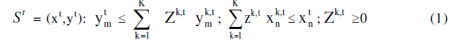 |
| Which exhibits constant returns to scale and strong disposability of inputs and outputs [10]. Following [1], the assumption of CRS can be relaxed and one may allow for variable returns to scale by putting the following restriction in (1) [6]: |
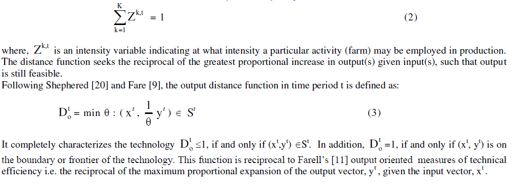 |
Calculation of Distance Function: A Linear Programming Problem |
 |
| The output distance function under VRS technology can be calculated by putting the restriction (2) in the above LP problem. |
| In this study, each farm is treated as a separate DMU (Decision making unit). The Number of DMUs k=474, for the study area of Bargarh district of Orissa. The number of inputs n=8, the number of outputs m=1. The decision variables are the shadow prices i.e., Z1, Z2 . . . Z474. The expansion factor is θ in the output-oriented model. We are required to maximise the objective function Do subject to respective constraint as given in the model. The model given in equation (4) is run separately for each DMU and as such 474 linear programming problems are solved to obtain the efficiency estimate of all the DMUs. |
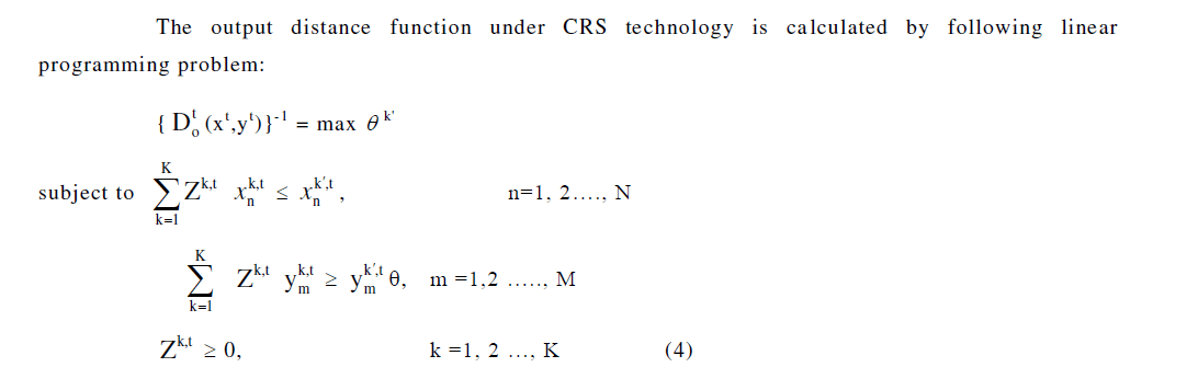
| Input Reducing (IR) BCC Model |
| The inefficient DMU can be made fully efficient by projection into a point on the envelopment surface. In the inputreducing model, the focus is on the maximal movement towards the frontier through proportional reduction of inputs. The output-increasing model focuses on the maximal movement towards the frontier through proportional augmentation of outputs. The linear programming problem for the BCC [6], input-reducing model is given as: |
 |
Artificial Neural Networks (ANNs): |
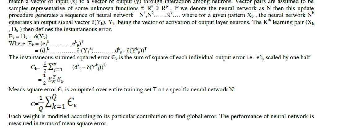
| Artificial Neural Network is a massively parallel distributed processing system made up of highly interconnected neural computing elements that have the ability to learn and thereby acquire knowledge and make it available for use. ANN can exhibit mapping capabilities i.e. they can map input pattern to their anticipated output pattern. |
| A neural network (NN), in general, is a highly interconnected network of a large number of processing elements (PEs) called neurons in an architecture. An NN can be massively parallel and therefore is said to exhibit mapping capabilities, that is, they can map input patterns to their associated output patterns. Neural Networks learn by examples. They can therefore be trained with known examples of a problem to ‘acquire’ knowledge about it. Once appropriately trained, the network can be put to effective use in solving ‘unknown’ or ‘untrained’ instances of the problem. |
| Neural networks adopt various learning mechanisms to enable NN to acquire knowledge. Supervised learning and unsupervised learning methods have turned out to be very popular. In supervised learning the network aims to minimize the error between the targeted (desired) output and the computed output to achieve better performance. However, in unsupervised learning, the network tries to learn by itself, organizing the input instances of the problems. |
| Neural networks have been successfully applied to problems in the field of pattern recognition, image processing, data comparison, forecasting and optimization to quote a few. |
Fitting Function: |
| Neural networks are good at fitting function as well as to recognize patterns. In fact there is proof that a simple neural network can fit any practical function. |
| For instance, we have data from agricultural farms. The present study aims to design a network that can predict the value of production of rice, given 8 pieces of expenditure of the farmers. We have 474 example of farmers for which we have those 8 items of data and associated with production(Y) value. |
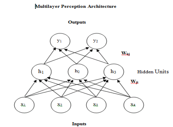
Multi-Layer Perceptron (MLP) |
| The general architecture shown below with three layers of neurons, the algorithm is extendable to networks with a large number of layers, input layer neurons are linear whereas neurons in hidden and output layers have sigmoidal signal function. Neuro solutions use back propagation of errors to train MLP. Back propagation uses gradient search and adjust weights contained in the network- this is how the network is trained. In our work we have considered input layer with eight neurons, hidden layer with two neurons and output with one neuron. The training of MLP is the process of learning to |
 |
 |
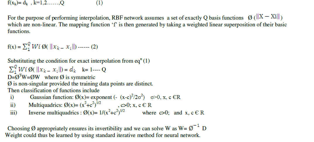
Radial Basis Function (RBF) Networks |
| RBFN is a feed forward neural networks that compete activations at the hidden neurons in a way that is different from what we do in feed forward neural network. Rather than employing an inner product between input vector and weight vector, hidden neuron activation in RBFN are completed using an exponential of a distance measure between the input vector and prototype vector that characterize a signal function at a hidden neuron. RBFN were introduced for the purpose of interpolation of data points on a finite data set. In an given training data set of input, output pair ζ= { xk, dk}Q Where k=1, XkÃÂÃâ Rn , dkÃÂÃâ R. Solving exact interpolation involves search of a mapping function that takes each input, Xk and maps its exactly into desired output dk : |
 |
Problem Definition: |
| To define a fitting problem for the toolbox, we have arranged a set of Q input vectors as columns in a XLs sheet. Then arrange another set of Q target vectors (the correct output vectors for each of input vectors in another column of same XLs sheet. |
| In Neuro Solution-6, to build neural network we have used Neural Builder. Neuro Builder presents a series of panels that represents logical steps in the neural network design process. Here, we can specify the neural network based on a particular neural model. |
Process of creating the model: |
| ïÃâ÷ The data in XLs sheet are tagged as desired and impute |
| ïÃâ÷ The neural network is designed by Neuro builder by selecting different parameters. |
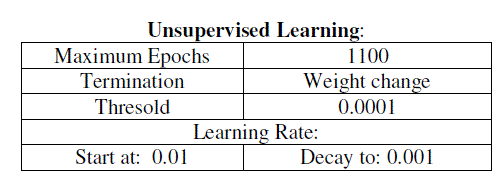
| ïÃâ÷ For RBF we selected and set |
| ïÃÆÃË Maximum Epochs to train |
| ïÃÆÃË Termination criteria for stopping the training |
| ïÃÆÃË Choose the frequency of weight update. |
| Neuro Solution-6, was employed to train the MLFANN. We processed the input and target data using appropriate scaling before training so that they fell within a certain range. The available observations were divided into three subsets. |
| i) Data set for training, which is used for evaluating gradiant and periodically updation of biases and weight of the network. We have taken 80% of total data set as training set. |
| ii) Second set of data is taken as cross-validation set. 15% of total data set is taken as cross-validation data set. |
| iii) To test the ANN, we used test data set which is 5% of total data set. |
| Besides this, we have also taken some datasets which missing the target value, as production data set. |
| MLFANN was trained using Gradiant Descent Algorithm (GDA). Many possibilities were observed. We have considered on hidden layer with input and output layer. The RBF was used for construction of Neural Network. |
 |
| This panel is used to specify unsupervised learning. |
 |
| It specifies the learning rate i.e. the amount to change the weights between epochs. |
Supervised Learning Control: |
| i. Maximum epoch specifies how many iterations (over the training set) will be done if no other criterion kicks on. |
| ii. It will terminate when there is minimum MSE on training set where threshold is 0. |
| iii. Once the network is has trained and we are ready to run our test set through the network, we may want to first load the best weight (the ones that produced the lowest error) obtained during the training. |
| iv. Batch learning updates the weights after the presentation of the entire training set. |
Cross-Validation and Test Set |
| ïÃâç The Cross-Validation (cv) set is used to determine the level of generalization produced by training set. CV is executed in occurance with training of the network. |
| ïÃâç The Testing set is used to test the performance of the network. Once the network has been trained, the weights are then frozen, the testing set is fed into the network and network output is compared with desired output. The testing is specified in the same manner as cv set. |
Performance Analysis |
| 1) MSE (Mean Square Error): |
| MSE should be as small as possible (i.e. approaches to zero) The MSE is an example of supervised learning, in which the learning rate is provided with a set of examples of desired network behaviour. |
| {P1, t1},{P1, t1}……….{PQ, tQ} |
| Here PQ is an input to the network and tQ is the corresponding target output. As each input applied to the network, the network output is compared to target. The error is calculated as the difference between the target output and network output. The goal is to minimize the average sum of the errors. |
 |
VI. METHODOLOGY RESULTS AND CONCLUSION |
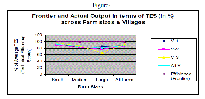
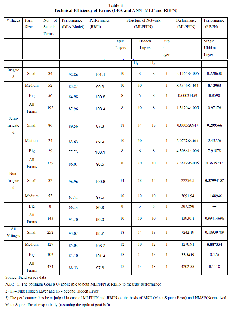
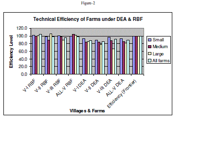
| The technical efficiency estimated across farm sizes and villages under study by DEA and ANN (MLPFFN and RBFN) models has been represented as follows. However, a detailed analysis of RBFN model and comparison of its result with DEA has been made. |
Technical Efficiency |
Findings from DEA |
| The BCC efficiency scores are evaluated for a number of individual farms under study for the agricultural year 2007-08. An efficiency score for each farm is computed relative to all other farms and itself. In other words, the efficiency of farm 1 for example is compared relative to efficiency characteristics of all other 473 observations in the given year. |
| The efficiency scores of all the farms in the sample so obtained are used to find out the average efficiency scores across different farm sizes and among different villages situated in different agro-climatic zones of the district under study. The over all averages have been calculated by using the weighted arithmetic mean. |
| The average technical efficiency scores vary across farm sizes and villages as evident from Figure-1 and Table-1. On an average the efficiency score varies from 81.01 per cent in large farms to 93.06% in case of small farms. Similarly, it varies from 86.07% in V-2 to 87.96% in V-1 and 91.69 in V-3. As observe from the table-1, the small farms are technically more efficient than those of medium and large farms in all the villages implying the fact that on an average, the realized output can be increased by 19%, 15% and 7% in case of large, medium and small farms respectively. Similarly it is around 12% in V-1, 14% in V-2, and 8% in V-3 respectively without any additional resources. Various factors may be responsible for the observed differences in efficiencies which need further analysis. |
 |
Findings from ANN (MLPFFN and RBFN) |
Findings from MLP |
| The simulations for MLP have been carried out with Mat Lab version 7.5 and the different simulations results are described in Experiment Sequence. The simulations are carried out to evaluate the efficiency of Back propagation Algorithm in multilayer perceptron network for predicting the production per acre. |
| The training and testing process for MLP have been carried out for around 60% and 20% of the sample data set respectively in each of the cases under study. These processes have also been undertaken on randomize data set. The best possible performance result (i.e. Value of MSE assuming the optimal goal is 0) pertaining the best fitted network structure in relation to the resultant hidden layers (H1 and H2 in this case) has been consider for the study. |
| It is observed from the table-1 that corresponding to the best suited network structure of MLP the performance result derived for medium farms in V-1 (i.e. MSE=8.63408e-011) is implying higher efficiency compared to that of small and big farms respectively. Similarly, the performance result (i.e. MSE=3.07376e-011) found for medium farms in V-2 shows higher efficiency compared to that of big and small farms respectively. The performance result (i.e. MSE=387.598) found for big farms in V-3 shows higher efficiency compared to that of medium and small farms respectively. The performance result (i.e. MSE=33.3419) found for big farms in All-V shows higher efficiency compared to that of medium and small farms respectively It can be inferred from the analysis that a direct relationship between the farm size and technical efficiency is persisting in V-3 and V-2 and All-V respectively. However V-I is found technically more efficient (i.e. MSE= 1.31294e-005) compared to that of V-2, V-3 and All-V respectively. On an average it is found from the MLP model that the deviation of actual output from the network output, given the inputs, is found much in case of All-V (entire area under study) as reflected by the performance result (i.e. MSE= 4202.55). This inference shows a technical inefficiency in the area under study even though the degree of inefficiency varies across farm sizes and villages under study. |
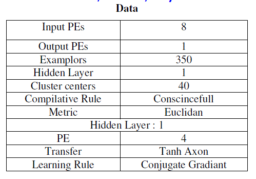
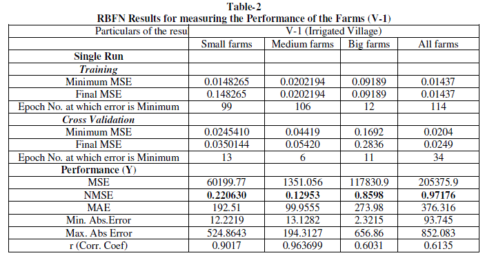
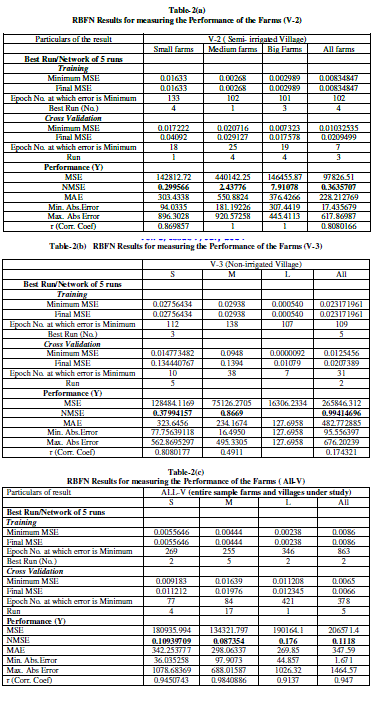
Findings from RBFN |
| The simulations for RBFN have been carried out with Neuro Solutions version 6.0 and the different simulations results are described in Experiment Sequence. The simulations are carried out to evaluate the efficiency of Back propagation Algorithm in RBF network for predicting the production per acre. |
| The training, cross-validation and testing process for RBFN have been carried out for around 55 to 65%, 15 to 20% and 10 to 15% of the sample data set respectively in each of the cases under study. These processes have also been undertaken on randomize data set. Single run and Multiple runs have also been made on the both original and random sample data set and the best fitted network results (i.e. the performance result based on the value of NMSE, assuming the optimal goal is 0) have been considered for the study. |
| It is observed from the table-1 that corresponding to the best suited performance result of the network derived for medium farms in V-1 (i.e. NMSE=0.12953) is implying higher efficiency compared to that of small and big farms respectively. Similarly, the performance result (i.e. NMSE=0.299566) found for Small farms in V-2 shows higher efficiency compared to that of medium and big farms respectively. The performance result (i.e. NMSE=0.37994157) found for Small farms in V- 3 shows higher efficiency compared to that of medium. In this case the result of big farms could not be worked out due to data insufficiency as the value of NMSE found was divisible by zero. The performance result (i.e. NMSE=0.087354) found for medium farms in All-V shows higher efficiency compared to that of small and big farms respectively It can be inferred from the analysis that there exists an inverse relationship between the farm size and technical efficiency is in V-2 and V-3. But the technical efficiency is found in favour of medium farms compared to other categories in V-3 and All-V. However V-2 is found technically more efficient (i.e. NMSE= 0.3635707) compared to that of V-1 and V-2. On an average it is found from the RBF model that the deviation of actual output from the network output, given the inputs, is found less compared that of MLP model in case of All-V (entire area under study) as reflected by the performance result RBF (i.e. NMSE= 0.1118). This inference also shows a technical inefficiency in the area under study even though the degree of inefficiency varies across farm sizes and villages under study. |
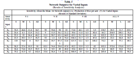
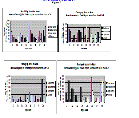
Findings of Sensitivity Analysis (based on RBFN model) |
| Sensitivity About the Mean for Network output(s) i.e. Production of Rice per acre (Y) for Varied inputs has been shown by the result of Standard Deviation as shown in Table-. In other words, the deviation of the inputs (corresponding to their network outputs) from the mean of their respective series has been shown by the result of standard deviation to analyze the sensitivity of the network outputs due to the degree of variation in the corresponding series of the inputs found for various farm sizes and villages under study. |
| The greater value of standard deviation ( σ) indicates that the value of Xi (input series X1 to X8 pertaining to their network outputs) are scattered widely away from the mean of their respective series. Thus a small value of standard deviation will imply that the distribution is homogeneous and a large value of standard deviation will imply that it is heterogeneous. It is observed from the analysis that on an average the network output is more sensitive to X5 for small and medium farms ( σ= 133 and 78.8 respectively), but X3 for big farms( σ=24-4) and X8 ( σ=102.8) for All farms in V-1 compared to other inputs in sequence as shown the table-3 . Similarly, on an average the network output is more sensitive to X6 for small and medium farms ( σ= 63.1 and 74.4 respectively), but X5 for big farms( σ=87.53) and X4 ( σ=76) for All farms in V-2, X8 for small farms ( σ=301), X1 for medium and big farms ( σ= 44.1 and 1.9 respectively ) and X5 ( σ=100) for All farms in V-3 compared to other inputs in sequence as shown the table- . In case of All-V, on an average the network output is sensitive to X8 for small and big farms ( σ= 269 and 322 respectively ), X6 for medium farms ( σ=372.6) and X1 for All farms ( σ=325.3) compared to other inputs in sequence as shown the table- |
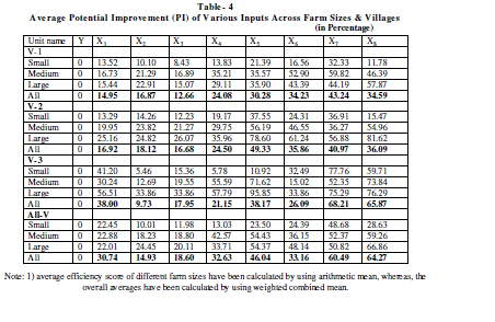
Potential Improvements of Inputs |
| The potential improvement of various inputs for 474 sample farms individually calculated based on the BCC (IR) model (i.e. output oriented measure of potential improvement of various inputs). The quantum of each input used excessively (i.e. the difference between the input use at Actual and Frontier level) has been worked out for each individual farm given the level of output and the result is compared across farm sizes and villages for policy implication at the end. |
| From this analysis it can be inferred that to produce a given level of output, how much input a farm is actually using, and how much the farm is ought to be used if he operates at frontier level. This provides the way of potential improvement to be done in the input usage to reach to its optimum usage. |
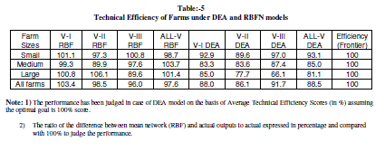
| A perusal of actual and frontier usage of inputs in the production of rice (Table-5) indicated that all the factors under consideration were used at levels higher than the frontier level by all the size groups. It also reveals that the percentage of excess inputs used in the production of rice increases with the increase in farm size. Further it is supported by our findings that the small farmers are technically more efficient than that of medium and large farms. Thus, the percentage of wastage of inputs is less in small farms in all the villages under study. But still there is scope for potential improvement in input usage by all size groups in all the villages. In other words, if the farms were technically efficient on an average they could have saved different inputs level: viz. X1, X2, X3, X4, X5, X6, X7 and X8 by 14.95, 16.87, 12.66, 24.08, 30.28, 34.23, 43.24 and 34.59 per cent respectively in V-1 (irrigated village). 16.92, 18.12, 16.68, 24.50, 49.33, 35.86, 40.97 and 36.09 per cent of the above said inputs respectively in V-2 (tailed irrigated village) and similarly 38, 9.73, 17.95, 27.15, 38.17, 26.09, 68.21 and 65.87 per cent respectively in V-3, 30.74, 14.93, 18.60, 32.63, 46.04, 33.16, 60.49 and 64.27 per cent of the said inputs respectively in All-V (case of entire sample) to achieve the current level of output. |
VII. CONCLUSION |
| Thus, from the foregoing analysis it is apparent that the resource use in rice cultivation in the study area leaves ample scope for improvement for all size groups in all the villages. Further, the medium and large farmers may be advised to achieve the resource-use efficiency effectively so as to raise their technical efficiency for realizing better output. By a better organisation of resources, a considerable amount of resources (i.e. inputs including land input) can be saved without affecting the achievement of the current level of production of rice per acre. Thus, the importance of productivity management in rice cultivation in terms of improving technical efficiency of the farmers by proper management and judicious utilisation of the resources is a matter of prime concerned today. Thus, it could be concluded that artificial neural network methodology is successful in describing the given data and can be used as a reliable tool for resource use optimization problems |
 |
 |
| 4) The performance has been judged in case of DEA model on the basis of Average Technical Efficiency Scores (in %) assuming the optimal goal is 100% score. |
 |
 |
 |
 |
 |
 |
 |
References |
|