Journal of Global Research in Computer Sciences
ISSN: 2229-371X
ISSN: 2229-371X
Chris Grassi*
Department of Mathematics and Computer Science, West Virginia University Institute of Technology, Beckley, USA
Received: 26-May-2023, Manuscript No. GRCS-23-99907; Editor assigned: 29-May-2023, Pre QC No. GRCS-23-99907(PQ); Reviewed: 13-Jun-2023, QC No. GRCS-23-99907; Revised: 20-Jun-2023, Manuscript No. GRCS-23-99907 (R); Published: 27-Jun-2023, DOI: 10.4172/2229-371X.14.4.001
Citation: Grassi C. Instability in the Centers of Radially Induced Subgraphs. J glob res comput sci. 2023;14:001
Copyright: © 2023 Grassi C. This is an open-access article distributed under the terms of the Creative Commons Attribution License, which permits unrestricted use, distribution, and reproduction in any medium, provided the original author and source are credited.
Centrality measures identify vertices that are potentially important when compared to the rest of the graph. When applied to an induced subgraph for which all vertices are within a given radius of the center, we sometimes find the center of the subgraph is different. Here, we provide some insight into how these “fulcrum” points can arise in graphs, and show that the degree to which the center can change is generally unbounded.
Visit for more related articles at Journal of Global Research in Computer Sciences
Centrality measures identify vertices that are potentially important when compared to the rest of the graph. When applied to an induced subgraph for which all vertices are within a given radius of the center, we sometimes find the center of the subgraph is different. Here, we provide some insight into how these “fulcrum” points can arise in graphs, and show that the degree to which the center can change is generally unbounded.
Path; Bipartite; Geodesic distance; Subgraph
This section is meant to give a dense yet concise list of definitions, many trivial, to many of the concepts, terms, and notations discussed further on. Fortunately, many simpler terms are intuitive enough that they should take little time to remember and others may already be known. More important definitions will be numbered by [section][index] to be easily referenced later. Yet more important definitions will be given in future sections where they will be applied and further discussed.
A graph is a pair G=(V, E) of sets satisfying E={{v1, v2} v1, v2 ∈ V }; thus the elements of E are 2-element subsets of V [1]. The elements of V are the nodes or vertices of the graph G and the elements of E are pairs of vertices and e is called an edge of G. If G contains a vertex v or an edge e, we write v ∈ G and e ∈ G respectively. If e=(v1, v2) is an ordered pair for all e ∈ G, then G is said to be a directed graph or digraph and v1 is called the start or initial and v2 is called the end or terminal of e. Otherwise, if all e ∈ G are unordered pairs, then G is said to be an undirected graph. From this point forward, all graphs are assumed to be undirected unless otherwise stated.
A vertex v is incident to an edge e if v ∈ e, and the degree of v, denoted deg(v), is the number of edges to which v is incident. Additionally, if G is a digraph, then the out degree, degout(v) is the number of edges in which v is the start, and the in degree, degin(v) is the number of edges in which v is the end.
For our first particularly notable definitions, we have a pair that go hand-in-hand with each other and will be implicitly referenced several times throughout the remainder of the paper.
Definition 1
A path in G=(V, E) from v0 to vk is an ordered set of distinct vertices P=(v0, v1, . . . , vk) ⊆ V such that vi=vj ⇔ i=j. The number of edges in P is called the length of P, written |P|.
Definition 2
The geodesic distance, or just distance, dG(v, w), is equal to min {|P| P is a path from v to w in G}.
When P is a shortest path between two vertices, we refer to P as a geodesic.
If there exists vertices v, w ∈ G such that there is no path1 from v to w, then we say G is disconnected; otherwise G is called a connected graph. If P={v0, v1, . . . , vk} is a path in G, except v0=vk, then we call P a cycle. Any graph with no cycles is called a forest and a connected forest is called a tree. In a tree, any vertex with a degree of 1 is called a leaf.
If  is a subgraph of G=(V, E) and we write
  [1]. An induced subgraph of G is a subgraph G′ such that every edge of G comprised only of vertices in G′ is itself in G′[2]; we write . We now introduce the concept of the radially induced subgraph.
Definition 3
Radially induced subgraph: Let G be a nonempty graph and H ⊆ G. Let x be a vertex in G. H is a radially induced subgraph about x with radius k, denoted H=G[x; k], if and only if for all vertices w ∈ G, w ∈ H if and only if dG(v, w) ≤ k.
Measures of centrality
Star graphs: In the subject of graph theory, a complete bipartite2 graph that is also a tree is called a “star”. The notable thing about star graphs is how they appear under different centrality measures. Star graphs were one of the primary motivators for finding more unanimously agreed upon metrics for graph centrality. That is, everyone agreed that the middle point of the star should serve as the most central vertex (Figure 1).

Figure 1: The star graph K3.
The only issue with agreeing what point is the center is determining what exactly gives that point its unique position. This gave prominence to the ideas on degree, betweenness, and closeness. For those three measures, the middle point achieves the highest ranking in all three cases [3]. In fact, the middle point of a star graph is at the same time:
1. The node with the highest degree,
2. The node with the smallest average distance to other nodes,
3. The node through which the most geodesics pass, and
4. The node that maximizes the dominant eigenvector of the adjacency matrix [4].
It’s these observations that lead to the conflicting ideas of centrality, which is why multiple independent measures are often used when analyzing a graph. Through the rest of this section, a handful of measures are discussed before moving on to applying one of them for the remainder of the paper.
Degree: One of the simpler measures available, degree centrality ranks vertices by their degrees. That is, vertices that connect to the most other vertices are considered to be the most “central” in the network. This measure comes from the idea that, the more nodes to which a vertex is adjacent, the more information it can receive or pass on in a shorter amount of time or distance [5].
For directed graphs, the in degree of a vertex can be considered its “prestige” or “popularity,” so the amount of nodes communicating directly with it, while its out degree can be viewed as its “influence,” how much information it can give to other nodes. Naturally, directed graphs make further distinction in regards to degree centrality, offering additional specification between in and out degrees.
Distance-based measures
Closeness: Closeness centrality is fairly to dissimilar degree centrality. Rather than considering only a node’s neighbours, closeness centrality takes into account every other node in the network. The formula for closeness is incredibly simple:
Closeness centrality is based on the distances between vertices. That is, the closer v is to every other vertex, the higher is closeness. A high closeness means that a vertex can quickly communicate with other vertices to give and receive information. Closeness centrality is the measure that we will be focusing on for the remainder of the paper.
Harmonic: This comparatively unpopular measure of centrality is neatly linked to closeness, in that it is also based on geodesic distance between vertices in Figure 2. The formula is also quite similar:

Figure 2: Most frequently used centrality measures. Harmonic centrality does not break top 10.
Harmonic centrality aims to solve a core issue with closeness: disconnected graphs. Under closeness centrality, a disconnected graph introduces an infinite term to the summation, causing the centrality of each vertex to be infinite. Harmonic centrality solves this by taking the reciprocal of the distance, and since 1/∞→0, disconnected graphs are of no issue. However, when considering a connected graph, or even just a connected component of a disconnected graph, closeness centrality is generally used more frequently in Figures 3a-3c.

Figure 3: The same graph shown with no centrality, harmonic, and closeness to compare. Note: (a) No highlights; (b)Harmonic centrality; (c) Closeness centrality.
Betweenness: Unlike other distance-based measures, betweenness centrality concerns itself not with the length of the geodesics; rather the number of them. In the case of betweenness, a vertex’s centrality is calculated by the fraction of geodesics between any two points, on which the vertex falls. That is,
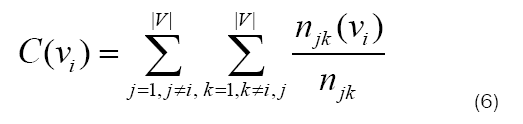
Where njk is the number of geodesics between vertices vj and vk, and njk(vi) is the number of such geodesics which contain vi [4].
The usefulness of this measure comes in calculating the probability that information sent between two vertices will pass through a given vertex. The intuitive meaning is that, if a large fraction of geodesics pass through v, then v must be important junction point in the network and severing that connection would cause a relatively large loss of information throughput and/or accessibility [7]. A large pitfall with betweenness centrality, however, is its computation time3. Typical betweenness computation algorithms have a time complexity of order O(n3), meaning the computation time increases significantly as more vertices enter the network (Figure 4 ) [8].

Figure 4: Example of the same graph with degree vs. eigenvector centrality [10].
Eigenvector: As an extension of simple degree centrality, eigenvector centrality serves to take into account both the number of connections of a node, as well as its relevance in terms of information flow [9]. Eigenvector centrality for a vertex vi is defined as
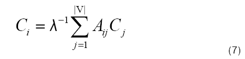
Where C is the eigenvector associated to the eigenvalue λ of the adjacency matrix A of graph G [9]. As opposed to degree centrality, eigenvector centrality incorporates the notion the important thing about having neighbors, is the importance of those neighbors themselves [5]. That is, having a lot of neighbors is nice, but if those neighbors are unimportant, they do not contribute much to the centrality score. Each vertex starts with an initial guess for its centrality, which is then used to compute a better score through equation 7. In the case of directed vs. undirected graphs, some complications arise in directed graphs (mainly the fact that the adjacency matrix is asymmetric) that make eigenvector centrality more useful in undirected graphs (Figure 4).
PageRank: It would be a mistake to not mention the centrality measure that is likely utilized by the most people daily-PageRank centrality, as Google named it. The improvement that PageRank seeks to make over eigenvector centrality is that eigenvector does not consider one important node pointing to many others. If one node is very important, does that make every node to which it points important as well? PageRank is similar to eigenvector centrality, but “the centrality derived from the graph neighbors is proportional to their centrality divided by their out-degree (Figures 5a-5c). Then vertices that point to many others pass only a small amount of centrality on to each of those others, even if their own centrality is high” [5].
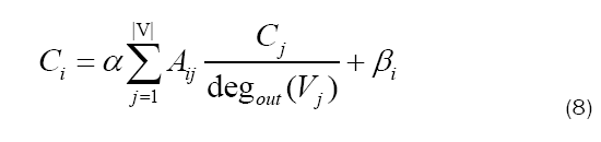

Figure 5a: Example of a social network comparing the eigenvector centrality vs. PageRank of a node (blue). Note: (a) Social network with no centrality applied.

Figure 5b: Example of a social network comparing the eigenvector centrality vs. PageRank of a node (blue). Note: (b) same social network with eigenvector centrality. Note the size (Relative centrality) of the blue vertex.

Figure 5c: Example of a social network comparing the eigenvector centrality vs. PageRank of a node (blue). Note: (c) same social network under page rank centrality.
Equation 8 contains a free parameter, α, which is chosen before computing the rankings4. As well, each term contains a bias βi to artificially increase or decrease the importance of a given node. It’s this system that makes Google search as effective a tool as it is.
Kite graph: In network analysis theory, the centrality of vertices is used to compare vertices in order to identify the “most important” vertices in the network [4]. Though extensive research has gone into finding worthwhile measures of centrality, there is no existing measure that is definitively “better” than any other- some measures are simply better for certain tasks than others are.
Popular approaches to centrality score based on geodesics, and others focus on a graph’s adjacency matrix. By these approaches, we often get vastly different results between centrality measures. Figures 6a-6d shows a graph created by David Krackhardt that displays how different centrality measures can give radically different results [12].

Figure 6: Krackhardt’s Kite Graph, showing different values for various measures in the same graph. Note: (a) Degree centrality; (b) Closeness centrality; (c) Harmonic centrality; (d) Betweenness centrality.
Fulcrums
Initially, the goal of this project was to discover if the center of a graph G could reveal anything about the center of its radially induced subgraphs. Intuitively speaking, it may make sense that if x is the center of G, then x is also the center of G[x, 0], G[x, 1], G[x, 2], . . . since closeness is a distance-based centrality measure.
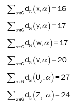
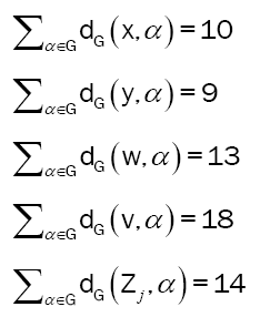
However, consider the graph in Figure 7. The total sum of distances, i.e. the reciprocal of the closeness, for each vertex has been given below. Notice how 1/C(x)=∑α∈G dG(x, α)=16 is less than all the others, meaning C(x) is greater than the others, and x is the center of G. Then look and see that 1/C(y)=9<1/C(x)=10. That means between G =G[x; 3] and G[x; 2], the center changes from x to y (Figures 8a-8d). This brings us to the “central” definition.
Sum of distances for vertices in Figures 7- 10.

Figure 7: A primitive fulcrum tree, G.

Figure 8: Radially induced subgraphs of G from Figure 7 with the center highlighted. Note: (a) G[x;0]; (b) G[x;1]; (c) G[x;2]; (d) G[x;3]

Figure 9: A primitive fulcrum tree F with ∆=7. Note: (a) F[x;7]; (b) F[x;8].

Figure 10: Process flowchart for constructing a basic fulcrum tree.
Sum of distances for vertices in G[x; 2]:
Definition 1: Fulcrum
Let G be a graph and let vertex x be the center of G by centrality measure C. If there exists at least one radius r such that x is not the center of G[x; r] by C, then we call G a fulcrum graph with respect to C, and x a fulcrum vertex (or fulcrum) of G.
The next question to explore is whether or not this “shift” is bounded, and if so, to what extent. It ends up being the case that it is not bounded. At least, not in a tree structure. In a tree, the distance which the center shifts is unbounded, even when we bound the maximum degree of all vertices. However, it is possible (and even worth further research) that enforcing the existence of, for example, a Hamilton cycle, would either bound the shift or remove it altogether. Nonetheless, in general, the magnitude of the shift, called µ from here on, is unbounded.
Constructing a fulcrum tree
A generalized fulcrum graph can be constructed algorithmically, defined by a singer parameter ∆ ≥ 4 as shown in Figure 10. Then, if F is a fulcrum tree with max degree ∆, we say F∈ F∆ where F∆ is the set of all fulcrum graphs with max degree ∆. Under such construction, we refer to the branch B∆ consisting of vertices v1, v2, . . . , v∆−1 as the principal branch, and all other branches B1, B2, . . . , B∆−1 as the non-principal or auxiliary branches. In addition, we refer to a fulcrum tree constructed from this process as a primitive fulcrum tree in Figures 9a and 9b.

Figure 11: Examples of each process in Figure 10.
Definition 2
If F∈F∆ is a fulcrum tree with shift equal to 1, we call it a primitive fulcrum tree.
Along with our maximum degree ∆, we can also use another parameter to construct a fulcrum tree. Recall that the “shift” of the center, µ, is unbounded. We can also use this parameter to create a distinct fulcrum tree. This idea leads us to the following proposition.
Proposition 1: Given ∆ ≥ 4 and µ ≥ 1, there exists a fulcrum tree with respect to closeness centrality  is the set of all fulcrum graphs with max degree ∆ and shift exactly equal to µ.
This process uses a modified construction algorithm when compared to the process in Figure 10. To start, we remove the extra offshoots on the principal branch, as they are no longer necessary. After that, we exponentially append vertices on either end, starting with the principal, until the center has shifted sufficiently. After that, we repeat that same process of exponential grown on the auxiliary branches until the center shifts back to where it started. This process, while providing a shift of exactly µ, makes it difficult to find a formula to easily compute the closeness of a given vertex. As such, we provide a weakening of proposition 1 (Figures 11a and 11f).
Proposition 2: Given ∆ ≥ 4 and ω ≥ 1, there exists a fulcrum tree with respect to closeness centrality  is the set of all fulcrum graphs with max degree ∆ and shift of at least ω (Figure 12).

Figure 12: Example of a fulcrum graph created from the process in Figure 10 with ∆=5.
This modified version allows us to construct a fulcrum tree with a predictable number of vertices, which may cause the shift to be larger than intended. The difference is that the number of leaves in the tree is symmetric across all branches, meaning it becomes much easier to derive equations yielding the exact closeness value for a given vertex. Importantly though, the original idea stays the same: the shift is unbounded. We then call the resulting fulcrum tree an unstable fulcrum tree.
Definition 3:
If  is a fulcrum tree and
  and has a shif t of µ ≥ ω, we call it an unstable fulcrum tree of order µ.
Quantifying a fulcrum
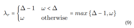
Before giving the equations, we must first name a handful of parameters. Recall ∆ is the maximum degree of the graph and ω is the minimum shift. We then define µ as the actual shift. Then we have λr, which represents the length of the branch on the principal branch. The value of λr is given by equation 9. From there, we then define λl as the length of the auxiliary branches by λl=λr+γ−1. This brings us to γ. The parameter γ represents the depth of the growth on the ends of each branch. That is, if we let m be the number of leaves in the tree, then γ=log∆−1 (m/∆).
You may notice, however, that this definition of γ relies on us already knowing the construction of the tree. As of the time of writing, it is unclear exactly what γ will be before constructing the graph. All that is known is that it grows proportionally with ω and inversely proportional with ∆ and γ ≥ 3 (Figures 13 and 14).

Figure 13: Fulcrum tree with ∆=4 showing the center (magenta) shift.

Figure 14: Values of γ correlated with ω and ∆.
Let be an unstable fulcrum tree, and refer to for the vertex labels (Figure 15). We then provide equations to calculate the closeness of any given vertex.

Figure 15: Labeling schema for an unstable fulcrum tree.
With these equations established, we now must prove that x is in fact the most central vertex in F. It is important to note beforehand that every parameter involved is a positive integer and, in particular, that ∆ ≥ 4 and γ ≥ 3.
Theorem 1
Given an unstable fulcrum graph  for all vertices
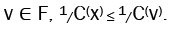 That is, x is the most central vertex in F.
Proof 1
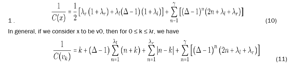
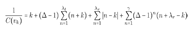
I. We first compare C(x) to C(vk). From equations 10 and 11, we have
Hence C(x) ≥ C(vk).
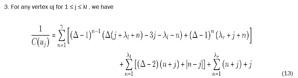
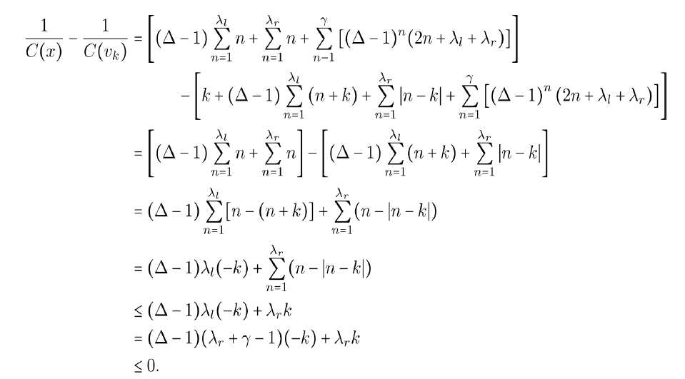
II. Now C(x) and C (uj).
Then, the values in each summation are less than or equal to zero. As such, their sum is less than or equal to zero and we have C(x) ≥ C(uj).
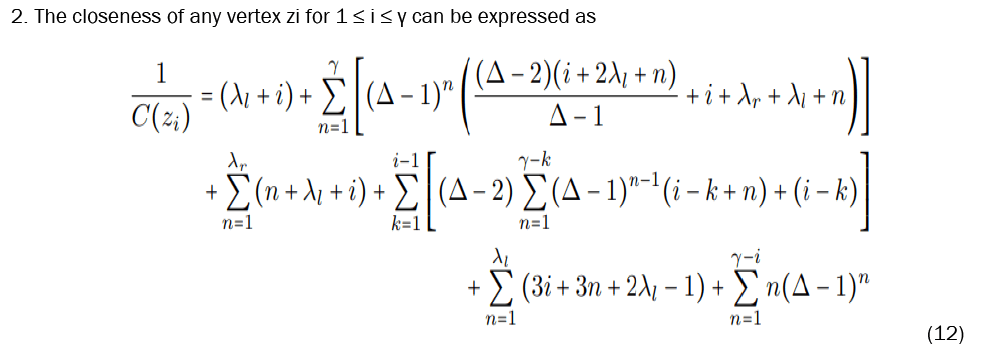
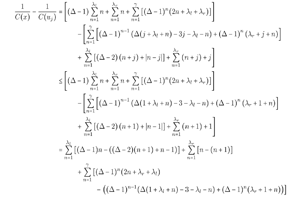
III. Next we look at C(x) and C(zi). Let an = n, bn = (∆ − 1)n(2n + λl + λr),cn,i = 3i + 3n + 2λl − 1, dn,i = n + λl + i,
and finally 
We can see then, that 
Thus 
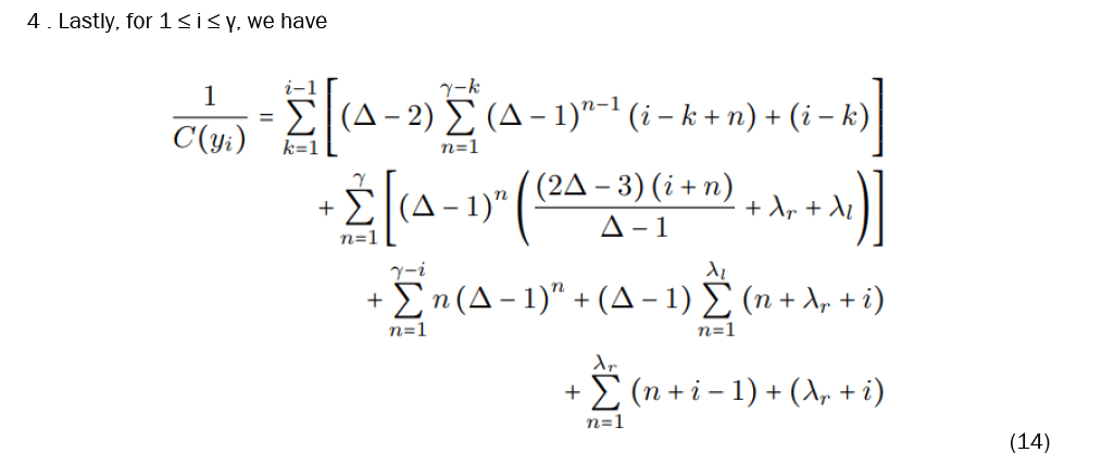
IV. Finally, we compare C(x) and C(yi). Similarly, we define an and bn the same way as in (iii), and then define
We then similarly have 
Therefore, x is the most central vertex in F.
Now that we have shown what the center of F is, we must now show that F is indeed a fulcrum graph. Recall definition 1. What this entails is finding some radius r such that x is not the center of F[x; r]. Thus we need not show what the center actually is; just that there is some vertex more central than x. So now we look back to proposition 2. As well as upgrading its status.
Theorem 2
Given ∆ ≥ 4 and ω ≥ 1, there exists a fulcrum tree 
Proof 2
In order to prove that F is a fulcrum tree, we need only prove that there is some radius r for which x is not the center of F[x; r]. However, for a stronger result, we can show a particular vertex is more central than x. But first, we must choose a radius. We note that the shift will be at its maximum with a radius of r=λl Thus the actual center, vµ, will be shifted at least as far as ω, and we need only prove that vω is more central than x.
We start by presenting a modified equation to calculate the closeness of vertices in this smaller induced subgraph. Notice that in F[x; λl], every vertex is present except for the vertices zi. Thus we can take the original equation, eq. (11), and simply subtract the contributions from zi.
We now show that 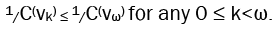
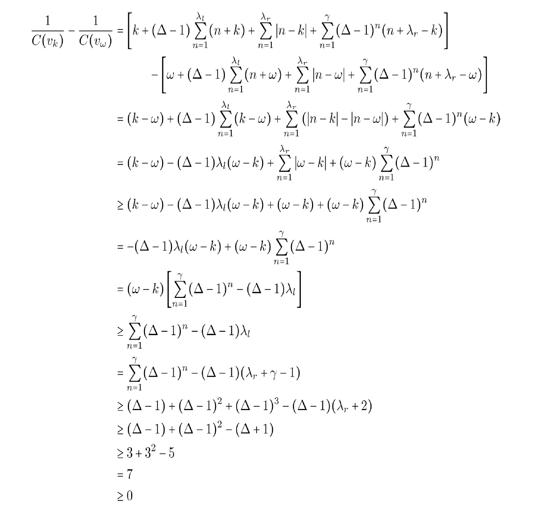
Therefore, we have 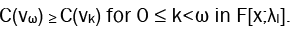
Remarks
Other examples of fulcrum graphs: The examples of fulcrum graphs shown here are not the only ones that exist. And other fulcrum graphs need not necessarily have such a well-defined, contrived structure. This graph, while being a fulcrum graph, is otherwise rather unremarkable. As another example, we can modify the kite graph shown in Figure 16a. By simply adding another vertex, we can construct a graph that not only is different from the previously discussed constructions, but also has more than one fulcrum. Figures 16a and 16b shows a graph in which both vertices f and g are fulcrums with respect to closeness centrality.

Figure 16: Modified kite graph showing two distinct fulcrums. Note: (a) Kite[f:3]=Kite[g:3]; (b) Kite[f:2]=Kite[g:2].
Definitions
1. We can also say that the distance from v to w is infinity, |P|= ∞.
2. That is, the graph can be partitioned into two sets of vertices V1, V2 where no edge has both endpoints in the same set.
3. “The computationally rather involved betweenness centrality index is the one most frequently employed in social network analysis. However, the sheer size of many instances occurring in practice makes the evaluation of betweenness centrality prohibitive” [8].
4. According to Mark Newman, Google uses α=0.85 [5]. Although it’s not clear that there is any rigorous theory behind this choice. More likely it is just a shrewd guess based on experimentation to find out what works well.
Further research opportunities
Currently, it is unknown whether or not fulcrum graphs exist with respect to centrality measures other than closeness. It seems reasonable to assume they do not exist under degree centrality, but other measures are worth further study. Something else to consider would be other ways to bind the shift of fulcrum graphs.
Also worth noting, is that the algorithm provided is only verified to work for a maximum degree of at least 4, and so it would require a special case to find a fulcrum tree with maximum degree of 3. But then perhaps it would be difficult to procedurally generate fulcrum trees in  for any such µ. Additionally, it can be trivially proven that fulcrum trees cannot exist with a max degree of less than 3.
In summary, this topic is largely unexplored, and I have covered only the surface. Additionally, the implications of these results are unknown in how they may or may not cause us to revisit the ways in which we look at centrality.
[Crossref] [Google Scholar] [PubMed]
[Crossref] [Google Scholar] [PubMed]