Journal of Global Research in Computer Sciences
ISSN: 2229-371X
ISSN: 2229-371X
Ahed Albadin*, Chadi Albitar, Assef Jafar
Department of Electrical Systems and Mechanical, Higher Institute for Applied Sciences and Technology (HIAST), Damascus, Syria
Received: 20-Dec-2021, Manuscript No. grcs-21-4736; Editor assigned: 22- Dec-2021, Pre QC No. grcs-21-4736 (PQ); Reviewed: 05- Jan-2022, QC No. grcs-21-4736; Accepted: 10-Jan-2022, Manuscript No. grcs-21-4736 (A); Published: 17-Jan-2022, DOI: 10.4172/ 2229-371X.13.1.005.
Visit for more related articles at Journal of Global Research in Computer Sciences
This paper introduces a modified algorithm of the Intelligent Trial and Error Algorithm (IT and E) to help the mobile robots to adapt to failure in a short time. Previous proposed algorithms do not require self-diagnosis as they perform training before the damage occurs. These algorithms do not take into consideration the quality of the chosen solution to overcome a failure. In order to determine a better solution, we developed the (IT and E) algorithm by adding a coefficient related to the distance between the robot’s position and the optimal trajectory. We present the results of the modified algorithm simulated on a mobile hexapod robot. The comparison proves the efficiency of the proposed enhancement which outperformed the last one by four times.
Robot damage recovery; Robotics; Artificial intelligence; Autonomous systems; Bayesian Optimization
With the development of science and research, and the existence of computer capabilities, it has become possible to improve AI and machine learning algorithms, whether in image processing or in the field of robotics. Many algorithms have been developed enabling legged robots to learn to walk or even learn a human demonstrated task without having prior knowledge of robot dynamics. These algorithms relied on Trial and Error, or Reinforcement Learning RL.
Robots are not only expected to adapt to the unknown environment, but also to adapt to possible failures in order to complete the task successfully. Recently, new algorithms have been studied that enable robots to diagnose the failure and then use a pre-prepared plan to bypass the failure[1]. Current robots cannot think on their own to find a behaviour that compensates for the failure, but rather need a pre-programed plan for each damage.
All robots have the risk to be damaged, especially those that have legs or have multiple motors. However, these robots depend on self-diagnosis and then choosing the best pre-programed plan[2]. This requires an accurate diagnosis and the presence of many sensors, which complicates the design of the robot, and it is also very difficult to find a solution for every possible damage as it is not possible to anticipate all faults. This approach fails with either a misdiagnosis or an inadequate pre- programed plan.
Instead of attempting to diagnose the failure, robots could adapt by trial-and- error, as it is the case of injured animals (e.g., learning which limb minimizes pain and thus reduces the use of this limb). This problem can be seen as a reinforcement learning problem, that is, when an engine fails, the robot tries to adapt and accomplish the task by maximizing a certain reward function aimed to deliver the robot to a new position or moving in a specific direction, i.e., robots with many legs (six legs) can balance on three legs, therefore, a damage in one leg should not affect walking.
Current algorithms are impractical due to the curse of dimensionality, and the irrational time needed to adapt. Calibration of one parameter usually requires 5 to 10 minutes, while some take several hours. This is unacceptable because it consumes a lot of energy, besides, successive testing may expose the robot to a new damage. In our article, we focus on studying the Intelligent Trial-and-Error (IT and E) algorithm for robot adaptation to failure without the need of self-diagnosis[3]. The proposed algorithm requires prior training before starting the adaptation process and it guarantees shorter time (less than a minute). The algorithm has been tested on an eight DoF robotic arm and on a hexapod robot. However, here we are trying to improve this algorithm and test the results by simulation on a mobile hexapod robot.
Related works
Several methods have been applied in the field of self-adaptation robots, most of the work has focused on reducing the time required to adapt. The IT and E algorithm has proven its effectiveness for various possible failures[3]. A map containing periodic pattern controllers was created and tested on the simulated robot. When a performance drop damage) occurs in the real robot, one of the controllers is selected in order to obtain the best performance, with the help of an optimization tool called Bayesian Optimization (BO). The previous method has been developed so that it can work without the need to return to the initial state (Reset-free Trial-and-Error algorithm)[4]. This algorithm allows complex robots to quickly recover from the damage while completing their tasks and taking the environment and obstacles into account. A model was also used to adapt by continuous comparison of the simulated robot with an undamaged model in order to detect changes that occurred as a result of the failure[5]. Another approach has focused on the adaptation of legged robots and implemented the adaptation using Central Pattern Generators (CPG)[6]. To overcome the problems of delays in sensors, motors, and noise, the texplore algorithm was used and it is the first algorithm to do so[7]. The algorithm relies on reinforcement learning method to learn the random forest model of the system. The algorithm presented in included the integration of IT and E (using a behaviour performance map) with Deep Reinforcement Learning DRL in order to train thousands of policies and store them in this map[8]. When damage or a change in the environment occurs, the best strategy is searched using Bayesian Optimization.
This article presents the IT and E algorithm that was chosen due to its simplicity compared to other methods. Previous algorithms do not take into account the quality of the proposed solution in terms of performance, so we propose to add a factor to choose the solution that takes into account the robot’s distance to the optimal path. We present this development for mobile robots (hexapod robot) and compare of results in terms of performance before and after adding the modification.
Modified IT and E algorithm.
The algorithm consists of two main phases: the behaviour performance map creation phase applied on the proper robot using MAP-Elites algorithm, and the adaptation phase for the damaged robot using (M-BOA Map-based Bayesian Optimization Algorithm)[9]. A large number of solutions are stored within a multi-dimensional map, and when certain damage occurs, the default solution becomes ineffective. Therefore, an optimal solution suitable for this situation is searched using Bayesian Optimization.
Map creation phase: The map contains high-performance solution in each location. Each location (co- ordinates) is reached by a behavioural descriptor that describes the general characteristics of this solution, and each solution has a specific performance. This map is called the behaviour performance map[3].
Building this map begins with the initialization step by generating random solutions. The descriptor of this solution and its performance is evaluated, and stored in its specific location in the map or replaced with another less performing one if the location is already occupied.
When the initialization phase is over, the algorithm will enter an iterative loop similar to population based methods such as evolutionary strategies. The stored solution is improved by random variation and selection. That is for each iteration, the algorithm randomly selects one of the solutions via a uniform distribution (all solutions have an equal chance to be selected). The algorithm will then take a copy of this solution and change one of its parameters to a random value. Its performance is measured and so its location, and its kept if it outperforms the current occupant at that location in the map.
Adaptation phase: The second phase starts when a drop in the performance occurs caused by damage. This phase accomplished by the Bayesian Optimization Algorithm that includes the previously created map (M-BOA).
The map is searched in order to find the solution that fits the new situation (the damage), using the Bayesian Optimization BO. The performance of the robot is evaluated at each stage of the algorithm, and is used to reevaluate the performance of the solutions stored within the map. BO searches for the maximum value of an unknown cost function. This gives the location of the solution with the highest performance. The algorithm creates a model for the cost function using regression method, and then this model is used to calculate the location of the new solution and to evaluate its performance, after that, the model is updated.
Gaussian process is used to update the cost function model, i.e., updating the performance of solutions stored within the map P(x) (where P expresses the behaviour performance map that stores the performance at each location x) adding uncertainty for each forecast. For a given number t of real evaluated performance samples P1: t = P1:t {P1...Pt} , the estimation of the performance function f at the new location xt+1 is represented by Gaussian distribution:

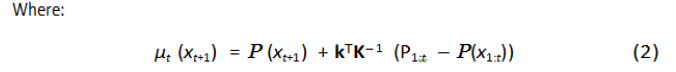

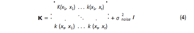

Where P(xt+1) is the expected performance for the sample t+1 (within simulation) taken from the map, and P1:t is the expected performance from the map for all tested samples. The term P1:t −P(x1:t) indicates the estimation of the difference between the actual performance and the expected one from the map. σ2 noise is a user defined noise, and k is the kernel function and it is the covariance function of the Gaussian process[10].
The prior belief is updated using the acquisition function based on the new observation. The role of this function is to drive the search of the optimal value and it is determined so that its optimal value is associated with the highest potential value of the cost function.
The UCB (Upper Confident Bound) function is used which gives the best results according to previous studies[11,12]. The function is given by the following relationship.

Where κ is a hyper-parameter for balancing exploration and exploitation
The first phase is applied within a computationally expensive simulation, but the second one is inexpensive, and it takes place in real time on the damaged robot, so this algorithm is relatively fast compared to other algorithms, and it does not depend on self-diagnosis.
The IT and E algorithm was tested on a hexapod robot through simulation and on a real platform. Unfortunately, the algorithm focused only on walking after the failure (the maximum distance traveled by the robot at the end of the simulation) and did not focus on the path that the robot takes during the movement.
Therefore, we suggested modifying the IT and E algorithm by adding a factor that expresses the robot’s distance to the optimal path (the straight line connecting the start and end point), and investing this factor in map creation phase, which helps this type of robots to obtain better performance. To end this, a new performance function was added to express the maximum distance minus the variance of the x-axis (the foreword direction) for a controller c, and it is defined as the following:
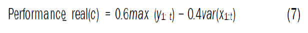
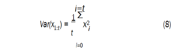
Where x1:t and y1:t the trajectories along the x-axis and y-axis for titrations. We notice from the previous equations that the performance function aims to maximize the distance on the y-axis and reduce the error on the x-axis. The weighted average was chosen (60% for the distance and 40% for the variance) according to the importance of the distances with respect to the variance and these are experimental parameters. In the following, we detail the steps of the application of the modified algorithm on a hexapod robot within a Matlab environment, and we compare the resulted performance before and after modification.
Experiment setup
We focused on studying the possibility of moving forward for a period of five seconds after damage occurs (losing one leg). Simulation environment was built in order to apply the two phases of the algorithm; hence, the process requires a dynamic environment that allows us to add links, friction, and collision with the ground. We chose to work in Matlab environment taking advantage of Sim Mechanics and Contact Forces library. Simulation was on a core i7 CPU 1.9 GHz RAM 16 GB computer.
The robot model was built in the simulation (Figure 1) in the form of a body connected to six legs; each leg consists of three revolute joints that are driven by a periodic controller that expresses joint angles. A position sensor is added to the body; also, a contact sensor is associated with each leg-end. Simulation can give the position of the robot (x, y) and the leg contacting with the ground (0,1).

Figure 1: The simulated robot.
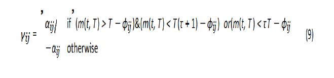
The angles of the joints are driven by a periodic function of time γ (t, α, ÃÂÃâ¢, τ) with a period of T=2s. This function is parameterized by its amplitude α, phase ÃÂÃâ¢, and duty cycle τ. We construct the function as follows:
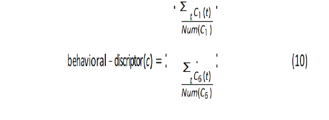
Where m is the mod function, i is the index of the leg, and j is the index of joint in leg i. The previous equation expresses the periodic trajectory of one of the joint’s angles within the domain [−αij, αij], which is inspired by legged animals, and then the trajectories is smoothed via a Gaussian filter. Initial values for these parameters are taken from 1, which expresses the tripod gait. Since the moment of leg touching the ground is known, the behavioural descriptor is chosen as a vector of six parameters, and each parameter expresses the percentage of the contact with the ground within the range [0,1] (0 contact, 1 no contact). The vector is expressed for a controller c as follows:
Where Ci is the percentage of the contact for leg i at the moment t, and Num (Ci) is the number of simulation steps, where the calculation is taken every 10 ms. There are several behavioral descriptors within [3], but the simpler one that can be practically applied is the one that relies on touching the ground, as touch sensors can be added at the end of the leg to enable the algorithm to calculate the percentage of the leg’s contact with the ground.
Map creation setup
We rely on the MAP-Elites algorithm in building the map. The algorithm starts by initializing the controller’s parameters in the map and the performance function, where the controller is assigned to the reference controller which is the tripod gait, and the performance function has a null value. For a specified number of iterations, a random controller is created for the first 1000 iterations and then the algorithm continues with the default steps.
The processing time for each iteration takes an average of 4 seconds, which is a very long for a million iterations. So we realized 300000 iterations and the MAP-Elites algorithm took two weeks (Figure 2).

Figure 2: The behavior-performance map.
Adaptation setup: After building the robot and the environment using SimMechanics and building the map, damage is applied and then the adaptation phase begins. For each iteration, a solution is applied (a controller), its performance is measured, and the Gaussian process is updated. The algorithm is repeated until it reaches a stage where it cannot find a controller that has better performance than its predecessor. When the performance expectation function μ is unable to predict better performance than the largest performance value obtained during experimentation, then the algorithm ends, and the ending condition is:

We also added an additional condition: if the previous condition is not met for a specified number of iterations (30), then the algorithm stops and the controller that gives the best experimental performance will be chosen. Best parameter values were chosen for the optimization from (σ2noise=0.01, ρ=0.1, κ=0.05); ρ is a hyper-parameter for the kernel function.
For each damage (losing a leg), 10 experiments were performed, and the mean, the standard deviation of the maximum performance, and the number of iterations required were measured.
Figures 3 and 4 show a comparison of two paths obtained for two experiments (adaptation after losing the first and third leg).

Figure 3: Comparison between the resulted paths a. after the modification and b. after losing the first leg before.

Figure 4: Comparison between the resulted paths a. after the modification and b. after losing the third leg before.
We found that the path had been improved significantly and it got close to a straight line. We must now compare the number of iterations needed to adapt between the two methods. Figure 5 shows that the number of iterations was not significantly affected by the modification despite additional restrictions, and in some cases it was even less than the previous algorithm. As for the maximum distance travelled on the forward direction (performance). Figure 6 presents a comparison between the two methods. We notice that the proposed modification in some cases approached the previous values and surpassed them. However, we can say that the adaptation algorithm after adding the modification gave better results than the previous one.

Figure 5: Comparison of the number of iterations needed to adapt before and after the modification.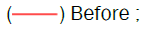


Figure 6: Comparison of the maximum distance traveled forward (performance) before and after the modification. 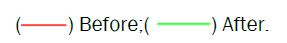
Finally, we compared the variance on the x-axis and found that the algorithm after adding the modification has significantly outperformed the algorithm applied in 1, and we also note that if we compare the mean variance (for all cases) before and after the modification, we will notice that the algorithm was improved by four times as shown in Figure 7.

Figure 7: Comparison of variance on the x-axis before and after adding the modification.
Mobile robots, especially those equipped with many legs, need algorithms that adapt to potential damages. These algorithms have been studied recently, but most of them took a long time to adapt and some needed selfdiagnosis.
One of the most important algorithms that require a short time to adapt and which depends on prior training (before the damage occurs) and on investing the training process in adapting to the failure are IT and E and MMPRL. The IT and E algorithm has been studied which uses Bayesian optimization to search for the best solution to adapt, and it depends on two main phases: map creation phase and adaptation phase.
We noticed that the algorithm in the case of hexapod robot focused only on reaching a successful walking after the damage, even if the path deviates from the robot’s forward direction. Our contribution was in the performance function. Better results were obtained for the trajectory, and thus the modified algorithm outperformed the previous one by four times, with about the same number of iterations needed to adapt.
We were successfully able to modify the proposed algorithm in terms of the trajectory of movement, but when the robot moves to a new location or towards another direction, the algorithm will re-adapt again. However, the successful adaptation reduces the use of the affected limb, and this can be invested later to make the robot predict its new model to avoid re-adaptation.
I would like to express my sincere gratitude to my advisors Prof. Chadi ALBITAR and Prof. Assef JAFAR for the continuous support of my Master study and research paper. Also, for their patience and motivation.