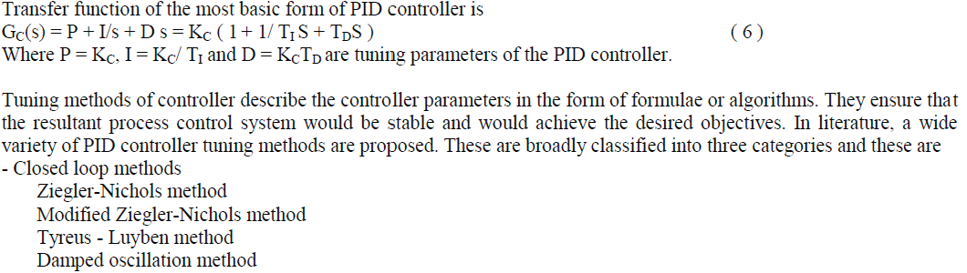
Automatic controllers are introduced for efficient control of the process industries. Proportional, Integral and derivative (PID) controllers are the most widely used controllers in the most process industries because of their robustness, easy implementation and simplicity. Various tuning methods like Ziegler-Nichols (Z-N) method, Cohen- Coon(C-C) method, Minimum error integral criteria method and Genetic Algorithms (GAs) have been suggested for optimum setting of PID controller parameters. In this paper the performance of Genetic algorithm based PID controller is compared with conventional PID controller for various tuning techniques in the case of three tank level process control system. This comparative study is carried out for set point tracking of three tank level process using computer simulation.
Keywords |
| PID controller, Ziegler-Nichols, Cohen-Coon, ISE, ITAE, IAE, Genetic Algorithm, Level process |
INTRODUCTION |
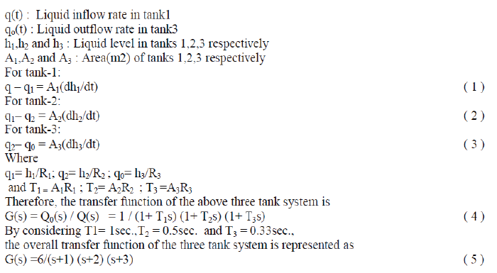
| In many industrial process applications the liquid level control is of much importance, especially in oil and gas
industries, waste water treatment plant & food processing industries. Three tank system relates to liquid level control
problems generally existing in industrial surge tanks. For example, accurate mould level control in continuous bloom
casting gained substantial benefits in steel producing companies [1].The general objective of the three tank level is to
track the set point and stabilize the level in the tanks with less number of oscillations and minimum settling time. The
final product quality depends on the accuracy of the level controller. The objective of the controller is to reach the
target and be able to track a new set point values quickly. This control problem can be solved by a number of level
control strategies ranging from conventional PID to Genetic algorithm based PID controllers[2],[3],[4].In level control
applications the conventional Proportional-Integral-Derivative (PID) controller is generally used, but the tuning
parameters of the controllers must be estimated by tuning technique either in frequency response or time response to
attain the desired performances[5],[6].Many different tuning techniques have been proposed for attaining the desired
control system response. These tuning techniques are developed based on one or more than one of the control
objectives as selected criterion. Many new techniques are proposed by the academic control community. One new
technique is Genetic Algorithm based tuning [7]. An advantage of the GA for auto tuning is that it does not need
gradient information. With this advantage Genetic Algorithm (GA) based PID controller is presently implemented in
many industrial automation applications [8]. |
| The paper has been organized as follows: Section 2 describes the modeling of three tank system. Section 3 reviews
various tuning methods of PID controller. Section 4 presents simulation of the process and PID controller for different
tuning methods. |
MODELING OF A THREE TANK LEVEL CONTROL PROCESS |
| Three first order processes are connected in series behaves as a three tank liquid level system, and its structure is shown
in Fig.1. |
 |
PID CONTROLLER TUNING METHODS |
 |
| - Open loop methods |
| Cohen and Coon method |
| Fertik method |
| IMC method |
| Minimum error criteria (IAE, ISE, ITAE) method |
| - Soft computing methods |
| Fuzzy Logic |
| Artificial Intelligence |
| Genetic Algorithm |
| Evolutionary Programming |
| In Closed loop tuning methods the plant is operating in closed loop and controller tuning is performed during automatic
state .In contrast the open loop techniques operate the plant in open loop and the controller tuning is done in manual
state. In soft computing methods, tuning parameters are estimated based on the guiding principles i.e. uncertainty,
tractability achievement approximation, robustness and minimum solution cost. In this paper the tuning methods
considered for simulation are
Ziegler-Nichols method, Cohen and Coon method, Minimum error criteria (IAE, ISE, ITAE) method and Genetic
Algorithm (GA) based tuning. |
| Ziegler-Nichols method: Ziegler-Nichols (ZN) tuning rule was the first tuning rule to provide a practical approach for
PID controller tuning. Based on the rule, a PID controller is tuned by firstly setting it to the Proportional-only mode but
varying the gain to make the process system in continuous oscillation (the edge of the stability).The corresponding gain
is called as the ultimate gain Ku and the oscillation period is denoted as the ultimate period Pu. |
| A Simulink model for closed loop process with P-control is simulated to determine the above parameters. The ultimate
gain Ku and the ultimate period Pu are also calculated analytically using Routh array. The key step of the Ziegler-
Nichols tuning approach is to estimate the ultimate gain and period [9]. Then, the controller tuning parameters (P,I,D)
are calculated from Ku and Pu using the Ziegler-Nichols tuning Table I. |
| Cohen and Coon method: In this method control action is removed and an open loop transient is introduced by a unit
step change in the signal to the process. At the output of the measuring element the step response is recorded
which is called as process reaction curve as shown in Figure 2.Then the dynamics of process is approximated by a first
order plus transportation lag model, with following parameters |
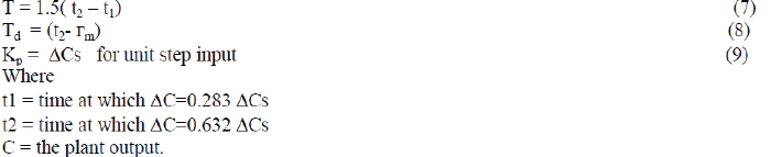 |
| This technique that published by Dr C. L. Smith [10] gives a better approximation to process reaction curve by first
order plus transportation lag process After estimation of three parameters of kp , T and Td, the tuning parameters can be
obtained, using Cohen-Coon [11] relations given in Table II. These relations were derived empirically to provide closed
loop response with a ¼ decay ratio. A Simulink model for open loop system is simulated for unit step input and kp , T
and Td are determined from the open loop response. |
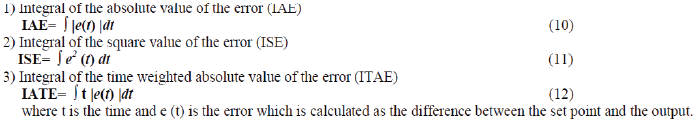
| Minimum error criteria (IAE, ISE, ITAE) method: As mentioned before tuning for ¼ decay ratio often leads to
oscillatory responses and also this criterion is developed by considering the closed loop response only at two points(the
first two peaks). Another approach is to introduce controller design relation based on a performance index that
considers the entire closed loop response. Some of the performance indices are |
 |
| Procedure to determine Controller tuning parameters: The following steps are taken to design PID controllers using the
minimum error criteria (ISE, IAE, and IATE). |
| i) The three tank process model including the controller algorithms in Simulink is developed |
| ii) A matlab m-file with an objective function that calculates the minimum error criteria is created. |
| iii) A function of matlab optimization toolbox is used to minimize the minimum error criteria. |
| On each evaluation of the objective function, the process model develop in the Simulink is executed and the specified
performance index and the corresponding tuning parameters (P, I, D) are determined using Simpson’s 1/3 rule [12]. |
| Genetic Algorithm (GA) based tuning: The genetic algorithm is an optimization technique that fulfills a parallel,
stochastic, but directed search to determine the fittest population. The GA-PID controller consists of a conventional
PID controller with its parameter optimized by genetic algorithm. By executing the following three steps Genetic
algorithm breeds computer programs to solve optimization problems. |
| 1) An initial population of compositions of the functions and terminals of the optimization problem is generated |
| 2) Perform the following sub steps iteratively on the population of programs until the criterion for the termination has
been achieved: |
| a) Each program in the population is executed and fitness value using the fitness measure is applied. |
| b) A new population of programs is created by applying the following operations. |
| Reproduction |
| Crossover |
| Mutation |
| 3) The identified individual program is designated by result designation (e.g., the best-so far individual). This result
may be a solution (or an approximate solution) to the problem. The specification of the designed GA technique is
shown in Table III. |
| Figure 3 shows the flowchart of the parameter optimizing procedure using GA. For details of genetic operators and
each block in the flowchart, one may consult literature [13][14][15].A matlab m-file is developed based on Genetic
algorithm with the specifications given in Table III. Optimum values of controller tuning parameters with respect to
time are estimated by executing the matlab file. |
SIMULATION RESULTS |
| Figure 4 depicts the process model developed in Simulink to simulate the three tank process control system using trial
and error method; the optimum tuning parameters of the controller in z-n and c-c methods are estimated from the
simulation results of Simulink diagram. In minimum error criteria method(IAE,ISE,ISTE) optimum tuning parameters are estimated by declaring tuning parameters(P,I,D ) of controller in Simulink as global variables and executing the
matlab file which invokes a function fminseasrch from matlab optimization toolbox[16]. The controller tuning
parameters estimated by Ziegler-Nichols, Cohen-Coon and minimum error criteria (IAE, ISE, IATE) methods are listed
in table III. The GA based PID controller tuning parameters are estimated using matlab file and the obtained tuning
parameters are shown in Figure 5. |
| With these tuning parameters Comparison results obtained for P,PI and PID controllers by Ziegler –Nichols and Cohen
–Coon methods for the three tank level processes for a unit step change in set point are shown in figures 6(a) and 6(b)
respectively and the corresponding time domain specifications are listed in tables IV and V. In both tuning methods,
PID controller gave better performance compared to P and PI controllers with reference to settling time, rise time,
offset, ISE, IAE and IATE. Compared to Ziegler –Nichols and Cohen-Coon methods PID controller gave better
performance in Ziegler-Nichols tuning method. Similarly with optimum tuning parameters the system responses for
unit step input for remaining tuning methods are shown in figures 6(c) to 6(f). For comparison purpose the performance
indices of three tank level process for unit step input by various PID tuning methods are listed in table VI. The
simulation results indicate that unit step response presents better performance using GA based PID tuning method
compared to other tuning methods.GA based tuning method gave minimum peak overshoot, minimum settling time and
less integral square error. |
CONCLUSION |
| Optimum tuning parameters of PID controller are estimated by six tuning methods (Z-N method, C-C method, ISE,
IAE, IATE and GA based PID method) for three tank level process for using Matlab/Simulink. Simulated results show
that GA based PID controller results in quick response with smaller peak overshoot and integral square error.
Moreover, this method has good ability to adapt to the tuning parameters for changes in process dynamics. To
summarize, the GA based PID controller has been proved to be an efficient method in the three tank level control
process. This method can be also used in a variety of non linear process control systems with large transportation lag
processes. This paper will be extend in future to the evolutionary algorithms to determine optimum PID tuning
parameters. |
| |
Tables at a glance |
 |
|
|
|
| Table 1 |
Table 2 |
Table 3 |
Table 4 |
| |
|
|
|
| Table 5 |
Table 6 |
Table 7 |
|
| |
Figures at a glance |
 |
 |
 |
 |
 |
| Figure 1 |
Figure 2 |
Figure 3 |
Figure 4 |
Figure 5 |
| |
 |
 |
 |
 |
 |
| Figure 6a |
Figure 6b |
Figure 6c |
Figure 6d |
Figure 6e |
| |
 |
| Figure 6f |
|
| |
References |
- Graebe S.F., Goodwin G.C., “Control Design and Implementation in Continuous Steel Casting”, IEEE Control Systems, August 1995, pp.64-71.
- Cheung Tak-Fal, LuybenW.L.,”Liquid Level Control in Single Tanks and Cascade of Tanks with Proportional-only and Proportional – Integral Feedback controllers”,Ind.Eng.Chem.Fundamentals,vol.18, No.1,1979,pp. 15-2.
- Astrom, K., T. Hagglund, “PID Controllers; Theory, Design and Tuning”, Instrument Society of America, Research Triangle Park, 1995.
- S.N.Sivanandam, S.N.Deepa, “Introduction to Genetic Algorithms”, Springer Publications Co., 2010.
- J.G.Ziegler and N.B.Nichols, “Optimum settings for automatic controller”, ASME Trans, Vol64, 1942, pp.759-768.
- W.K.Ho.C.C.Hang. and J.H.Zhou,”performance and gain and phase margins of well-known PI tuning formulas”, IEEE Transaction. ControlsystemsTechnology, 1995.
- D. E. Goldberg, “Genetic Algorithms in Search, Optimization, and Machine Learning”, Addison-Wesley Publishing Co., Inc., 1989.
- A.H.Jones and M.L.Tatnall,”Online frequency domain Identification for Genetic tuning of PI Controllers”, Proceedings of ICSE, Coventry,1994.
- J. G. Ziegler and N. B. Nichols, “Optimum settings for Automatic Controllers”, ASME Transactions, vol. 64, pp. 759–768, 1942.
- Smith, C.A., A.B. Copripio;”Principles and Practice of Automatic Process Control”, John Wiley & Sons, 1985.
- Seborg, D.E., T.F. Edgar, D.A.Mellichamp; “Process Dynamics and Control”, John Wiley & sons, 1989.
- S.C.Chapra and R.P.Canale., “Numerical Methods for Engineers”, McGraw-Hill International Edition, New York, 1998.
- L.Hao, C. L. Ma and F. Li, “Study of Adaptive PID Controller Based on Single Neuron and Genetic Optimization”, The 8th InternationalConference on Electronic Measurement and Instruments ICEMI, Vol. 1, 2007, pp. 240-243.
- R. Koza, F. H. Bennett, A. David and K. Martin, “A Genetic Programming III: Darwinian Invention and Problem Solving”, Morgan
- Kaufmann, San Francisco, 1999. C. R. Reeves, “Using Genetic Algorithms with Small Populations”, Proceedings of the 5th International Con-ference on Genetic Algorithms,1993.
- F.G.Martins, “Tuning PID controllers using the ITAE criterion”, International Journal Engineering Edition, vol.21, No.3, 2005
|