Yared Gurmu1*, Jing Qian2 and Victor De Gruttola3
1Division of Cardiovascular Medicine, Harvard Medical School, USA
2Department of Biostatistics and Epidemiology, University of Massachusetts, USA
3Department of Biostatistics, Harvard T.H. Chan School of Public Health, USA
Received Date: 17/01/2018 Accepted Date: 10/05/2018 Published Date: 18/05/2018
Visit for more related articles at Research & Reviews: Journal of Statistics and Mathematical Sciences
Partnership duration data are commonly obtained through surveys that collect information on relationships that are ongoing during a fixed time window. This sampling mechanism leads to duration data that are left truncated and right censored; such data have been analysed using the standard truncation product limit estimator (TPLE). In this paper, we describe a common sampling scheme for collecting sexual partnership data, discuss a key assumption required for the TPLE to be unbiased, and provide the conditions under which the nonparametric maximum likelihood estimator of the relationship duration distribution is unique and consistent. We also investigate the conditions required for the consistency of the regression coefcient from a Cox proportional hazards model that apply even when the distribution of duration is not completely identifiable due to restrictions on the support of the truncation distribution. Lastly, we will provide some illustrative examples on estimating distribution of most recent partnerships and present spline regression results based on partnership data collected from sexual behavior survey in Mochudi, Botswana.
Truncation product limit estimator; Partnership duration sampling; Left truncation; Right censoring; Consistent estimation
Estimating the duration of sexual partnerships is important in investigation of the epidemic dynamics of sexually transmitted infections (STI). Duration of such partnerships is a key feature in mathematical models of STIs and has been shown to be an important predictor of STI risk and of concurrency [1,2]. Goodreau et al. [3] utilize data on duration to model sexual partnership networks in their study of the roles of acute infection and concurrent partnerships in HIV transmission dynamics. Wang et al. [4] used duration in modeling spread of HIV for the purpose of designing intervention studies. In a different application of duration information, Matson et al. [1] investigated the association between concurrency and duration of relationships based on a prospective cohort that followed participants every six months. Using a multilevel mixed effect logistic regression, the study found that odds of concurrency (OR = 1.03, 95 % CI: [1.02,1.11]) increased with length of relationship. Distributions of duration of relationships are often estimated retrospectively from surveys that collect information about the length of partnerships that are ongoing or have ended within a fixed period (typically 6 months or a year) before the date of the survey. This form of sampling yields data that are left truncated (because the relationship had to have endured long enough to be present within the time window before the survey) and potentially right censored, should the relationship be ongoing at the time of the survey. Several authors have considered the problem of right censoring and left truncation (RCLT) in analysis of survival or failure-time data. For right-censored observations, the survival time lies in an interval of the form [C,∞] where C is the censoring time. In contrast, left truncation arises from sampling of observations conditional on the failure time itself. Denoting T as the left truncation time and X as the survival time, X is observable only if X > T. All observations on subjects for whom X < T are excluded from the observation process.
A common approach to account for right censoring and left truncation present in partnership duration data utilizes the truncation product limit estimator (TPLE), the left truncated version of the Kaplan Meier estimator [5]. The TPLE assigns non-zero mass only at event times as does the standard Kaplan-Meier estimator. By assigning mass in this way, the TPLE makes the additional assumption that no probability mass need be placed in intervals that lie between the left endpoint of a censoring interval and the left endpoint of a truncating interval (see figure 2). Assigning zero mass to such intervals avoids the problem of having multiple maxima of the nonparametric likelihood and thereby simplifies estimation. However, Frydman [6] demonstrated that consistent estimation may require mass to be placed in regions where the TPLE does not do so. Frydman modified Turnbull’s nonparametric estimator of the distribution function so that it correctly accommodates interval-censored and truncated data [7]. She showed that the support depends not only on the censoring intervals, as Turnbull [7] described, but also on the truncation intervals. Therefore, the implications of assumptions that restrict the support of the NPMLE, as does the TPLE, require more consideration. Further discussion illustrating the differences between the TPLE and Turnbull’s estimator with Frydman’s correction (TEFC) will be presented in later sections. The primary aims of this paper are to identify sampling conditions necessary to obtain a consistent estimator of the distribution of partnership durations from retrospectively collected survey data and to apply these insights to an analysis of the relationship duration distribution. The paper is organized as follows. The next section describes a common sampling scheme for collecting partnership duration data. Section 3 discusses the conditions under which the NPMLE of the relationship duration distribution for RCLT data is unique and consistent. We present the conditions regarding the size of the sampling window and the censoring and truncation time distributions that are necessary for the TPLE to be consistent. Section 4 presents conditions for consistency of parameter estimates from a Cox proportional hazards model where distribution of duration is not completely identifiable due to restrictions on the support of the truncation distribution. Section 5 examines the validity of a key assumption–the quasi-independence of truncation time and failure time–that is also necessary for consistency of the TPLE from RCLT data. This section also discusses a spline regression model. Section 6 provides a discussion.
Sampling Schemes for Partnership Data
Partnership surveys may collect information on a fixed number of most recent relationships or, alternatively, information may be collected on all relationships that are ongoing during a fixed time window called the sampling window [5]. In such partnership surveys, participants are repeatedly interviewed to provide detailed information regarding their prior partnerships including age at sexual debut as well as start and end time of their sexual partnerships. This general method of collecting cross-sectional partnership duration yields data that are length-biased, as longer relationships are more likely to be observed. One can avoid this observation bias only by prospectively following participants over their lifetime starting from the time of their sexual debut. Such a design would provide incident sampling that allows complete observation of partnerships, but is obviously infeasible.
We note that this sampling scheme for partnership studies often combines prevalent and incident sampling. In our application dataset from a pilot study in Mochudi, Botswana, data are collected cross-sectionally among those whose relationships have been ongoing within the 12 month period before the interview date. Such prevalent sampling schemes do not generally obtain information about the time of initiation of partner ships that ended before the window described above; hence, the duration of such relationships are truncated. In contrast data on subjects who initiate partnerships after the left endpoint of the window are observed as in incident sampling. Estimates of the distribution using only the latter are unbiased, but are censored by the end of the sampling window and do not make full use of available information.
Statistical Notation for Relationship Data
Let Tf and Td represent the calendar time of relationship formation and dissolution, respectively, and let
τ represent the calendar time of interview. Tf and Td are considered random while the interview date τ is taken to be fixed. The relationship duration times are defined as X = Td−Tf. If the relationship is ongoing at the time of the interview (i.e. Td is after τ), the length of X is censored at C = τ−Tf, where C is known as the right censoring time. The observed duration variable is Y = min (X,C); we define δ = I(X ≤ C). The truncation time is defined as follows:

where w is the length of the sampling window. If X < T, we do not observe the relationship. See figure 1 for an illustration of the time course of partnerships and the sampling scheme.

Figure 1: Illustration of the time course of partnerships and the sampling scheme. Tf, Td and τ represent the calendar times of relationship formation, relationship dissolution, and interview, respectively. Partnerships ongoing within the sampling window, w, are observed; partnerships that end prior to the sampling window are not observed and therefore truncated. The sampling window (w) in this figure is 1 year (365 days). Relationship durations that end before τ −365 are not observed in the sampled data while relationship durations that end after τ are right censored.
observed data are assumed to be realizations of independent and identically distributed (iid) (Ti,Yi,δi) for i = 1,·· ,n that meet this sampling requirement. Note the special nature of the relationship between the truncation and censoring times, C = T + w for all truncated durations. Throughout the rest of the paper, we will assume X follows the distribution function F.
This section characterizes the support for the estimator of the distribution of duration, ˆ F, and investigates the conditions required for consistency in a variety of settings with discontinuities in the truncation and censoring distributions.
Turnbull’s Estimator with Frydman’s Correction (TEFC) and TPLE
Turnbull [7] developed a nonparametric estimator of the failure-time distribution function of random variable X for arbitrarily censored and truncated data. Truncation implies that independent observations are sampled from F(x) = Pr(X ≤ x|X ∈ Bi), where the set Bi is the truncation interval, defined as Bi = [Vi,Ui]. In the case of left truncation Bi = [Ti,∞). In addition, each Xi can be censored by Ai = [Li,Ri]. In the case of exact observations Xi = xi, we set Ai = [xi,xi]. For right censored data we have Ai = [Ci,∞). Note that the sets (Ai,Bi) are assumed to be independent of Xi. Turnbull’s likelihood (Turnbull 1976) for the observed data is given by
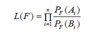
which can be simplified as
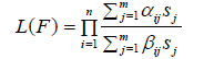 (1)
(1)
where αij =I([qj,pj] ∈ Ai) , βij =I([qj,pj] ∈ Bi), qj ∈ L =Sn i=1{Li,Ui}, pj ∈ R =Sn i=1{Ri,Vi}, sj = F(pj+)−F(qj−) and j ∈{1,·· ,m}.
Frydman [6] pointed out that the support of ˆ F is made up of the union of disjoint intervals [qj,pj].
Therefore, finding the NPMLE of F reduces to maximizing the likelihood in equation (1) with respect to s = (s1,·· ,sm). The constraints for maximization arePn i=1 sj = 1 and 0 ≤ sj ≤ 1. By construction the intervals [qj,pj] cannot contain any other members of R or L. Frydman’s characterization of the support applies in the general case of interval censored, grouped as well as truncated data. For the special case of partnership data which are left truncated and right censored, the support of can be simplified as follows:
1. for exactly observed relationship duration, say xi, we set qj = pj = xi.
2. for right censored observation that is immediately followed by a left truncated observation, we set qj = ci, and pj = vi provided ci < vi.
Note that in step (2), we obtain an interval where there could be non-zero mass. Henceforth, interval of this type will be re- ferred as region where events are not observable (RENO).
By contrast, the TPLE estimator for the survival function, S(x) = 1−F(x), is given by
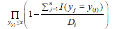
where Di =Pn j=1 I(tj ≤ y(i) ≤ yj), y(1),·· ,y(k) are distinct ordered observed failure times. From the form of the TPLE, it can be seen that the support of ˆ F is restricted to exact times of failure. Unlike the TPLE, Turnbull’s NPMLE with Frydman’s correction (TEFC) allows for placement of mass in RENO.
Example of disagreement between TEFC and and TPLE
We consider a simple numerical example to illustrate the difference between the support of the TEFC and TPLE. The data for the example are displayed in Figure 2. Partnership durations are reported from three individuals; two of them (observations 1 and 3 in the figure) are reported as x = 4 months and x = 9 months. These relationships are taken to be sampled conditional on being greater than 3 and 8 months, respectively. The censored relationship (observation 2) is reported to be at least 6 months and is sampled conditional on being greater than 1 month.

Figure 2: Example of disagreement between TEFC and TPLE for the partnership duration data (a) from three individuals. The support of the TEFC includes the shaded region from [6,8] in addition to the support of the TPLE {4,9} which is shown in figure 2(b). The line segments starting with ‘(’ correspond to the truncation interval for each observation. The portion of the line segment to the right of ‘[’ is the censoring interval. The shaded interval that lies between the left endpoint of the censoring interval for observation number 2 and the left endpoint of a truncating interval for observation number 3 is RENO.
As shown in figure 2(a), application of steps (1) and (2) from the previous section suggests that TEFC put mass at x = 4 and x = 9 as well as the shaded region, [6,8]. Note that the left and right endpoints of the shaded region are a right censored event time that is followed by a left truncation time with no intervening events; there is no guarantee of there being no mass in this region. From figure 2 (a), the shaded region reflects knowledge that the relationship duration is greater than 6 months for observation 1. However, observation 3 implies that relationship durations less than 8 months, the truncation time, are possible. The likelihood for this example is:
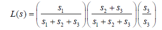 (2)
(2)
where s1,s2,and s3 are the masses at 4, [6,8], and 9, respectively. Since s1 + s2 + s3 = 1, the likelihood simplifies to L(s) = s1(s2 +s3), which is maximized at s1 = 1 2 and s2 +s3 = 1 2. TEFC is not unique for this simple problem as there are infinitely many s2 and s3 satisfying the above constraints. The TPLE shown in figure 2 (b) is obtained from the above likelihood by setting mass in the shaded region to 0 (i.e. s2 = 0).
Intrinsic versus Ignorable RENO and implications for consistency
In practice, relationship datasets that arise from surveys can have two types of RENO, both of which are formed between a right censored observation and the left truncation times that immediately follows it. An ignorable RENO has width that converges to 0 as n →∞; an intrinsic RENO does not. If the truncation distribution is continuous, the width of the RENO converges to 0 as n →∞, yielding ignorable RENO. For example the RENO shown in figure 2 can be considered as ignorable as the width of the RENO (i.e. the shaded region) converges to 0 as n →∞. However, as illustrated by figure 3, if the truncation distribution is discontinuous intrinsic RENOs can arise. In this setting, the support of X is continuous, the truncation support is discontinuous, and the censoring support is equal to the truncation support shifted by a fixed constant w < 0.5. The width of the RENO in this example approaches 0.5−w as n →∞; no values between 0.5+w and 1 are observable irrespective of the sample size. Any observation xi that falls within this window will either be censored to 0.5 + w if ti ∈ (0,0.5) or will be excluded if ti ∈ (1,1.5). In order to demonstrate this, we consider the case w = 0.1 and xi = 0.7. If the corresponding truncation time ti ∈ (0,0.5) then the corresponding ci ∈ (0.1,0.6) which implies our xi = 0.7 will be censored by min (0.7,ci) = ci. If the corresponding truncation time ti ∈ (1,1.5) then xi = 0.7 will not appear in our sample since xi < ti. In both cases, no observations can be made between 0.6 and 1 given the sampling window w = 0.1.

Figure 3: Example of Intrinsic RENO: X has continuous support but C and T do not. No duration values, xi, between .5 + w and 1 are observable whenever the size of the sampling window is smaller than the size of the discontinuity in the support of the truncation times (i.e. w ≤ .5).
Consistency of the TPLE when there is intrinsic RENO
The examples above illustrate why there can be no unique NPMLE in settings with at least one RENO. In addition, ˆ Stple(x) may not be a consistent estimator for the distribution of the duration variable when there are one or more RENOs. As illustrated by simulation in the next section, if a RENO exists between x1 and x2 then it is possible that
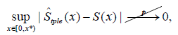
where x1 ≤ x2 < x8 and x8 lies in the interior of the support of the duration distribution function F and the censoring distribution function G. The latter condition is equivalent to 1−F(x*) > 0 and 1−G(x*) > 0, and hence F(x) > 0 and G(x) > 0 for 0 ≤ x ≤ x*. Nonetheless, ˆ Stple(x) has some useful asymptotic properties.
Theorem 3.1. Given the presence of a RENO between x1 and x2 and the conditions x1 ≤ x2 < x8, 1−F(x8) > 0 and 1−G(x8) > 0, ˆ Stple(x) is consistent for features of the distribution of S(x) as follows:
sup x∈[0,x1]|ˆ Stple(x)−S(x)| p → 0 and sup x∈(x2,x8)|ˆ Stple(x|x > x2)−S(x|x > x2)| p → 0
The proof is provided in the appendix and relies on the work of Tsai et al. [8] and Lai and Ying [9], who showed that the conditional distribution S(x|X > a) = P(X > x|X > a) can be estimated consistently for a ≤ X ≤ b, where a is the lower boundary on the support of the left truncation variable T and b is the upper boundary on the right-censoring variable C.
We use simulation to illustrate the conditions under which the TPLE is consistent in the presence of RENO. In order to create a suffciently large RENO, we will generate our dataset using the following procedure:
For durations subject to truncation (i.e. Ti > 0), truncation time is drawn from a mixture of two uniform distributions,
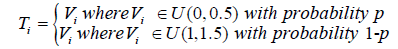
2. The duration variable will be sampled from the exponential distribution with CDF 1 − e−λx where λ {.25,.5,.75,1}. 3. If Xi ≥ Ti keep data. Otherwise, discard the data since it is not possible to observe it.
4. Repeat steps 1 and 2 until N 2 truncated subjects are obtained.
5. For durations not subject to truncation, truncation time is Ti = 0. About 50% or N 2 of the durations will not be subject to truncation as is the case in our dataset obtained from Mochudi, Botswana.
6. Generate the censoring times as
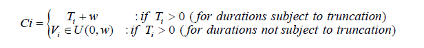
Ci = for i ∈{1,·· ,N} where w is the size of the sampling window.
7. Lastly, define Yi =min(Ci,Xi) and δi =I[Xi ≤ Ci].
The final dataset contains (Ti,Ci,Yi,δi) for i ∈ {1,·· ,N}. Note the width of the sampling window w is varied in order to control the size of the RENO and investigate its impact on consistency.
We consider the following set of parameters: λ = 0.25,N = 104 and w ∈ {.1,.2,·· ,1}. Figure 5 illustrates the diference between TPLE Stple(x) and S(x) and the impact of the size of the RENO. We can estimate S(x) unconditionally since the lower boundary of the support of the truncation times, τ8 = 0.
In addition, the simulations suggest that even if there are discontinuities in the truncation and censoring support, the TPLE will converge to the true distribution provided that there is not an intrinsic RENO. Thus, it is important to distinguish between discontinuities in the support of T and C that do and do not result in intrinsic RENOs. This distinction can be illustrated by comparing figure 3 and figure 4(a). In both, the support of C and T partially overlap, but intrinsic RENOs arise only in the setting displayed in Figure 3, because the setting of Figure 4(a) permits observation of duration of relationships that fall within the regions of discontinuity, namely [0.5,0.7] and [1.5,1.7]. Additional examples that illustrate the diference between ignorable and intrinsic RENOs are illustrated in figures 4(b) and 4(c).

Figure 4: Discontinuities that do not lead to RENOs are shown in figures (a) and (c). The discontinuity shown in (b) leads to intrinsic RENO as any xi ∈ (.5,1) is not observable.

Figure 5: Performance of TPLE (dashed line) in the Presence of RENO: λ = 0.25,N = 104 and w = .8,.7,.2,.1 for figures (a), (b),d (d), ctively. The true distribution of the relationship duration time is given by solid line. The vertical lines represent the boundaries of the RENO. An intrinsic RENO is present whenever the size of the sampling window is smaller than the size of the discontinuity in the support of the truncation times (i.e. w ≤ .5) as in (a) and (b).
We examine conditions for the consistency of the estimated regression parameter, ˆ β, from a Cox proportional hazards model. The Cox model assumes that the hazard function for X conditional on the covariate vector Z is given by
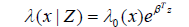
where βT is the vector of unknown coefcients and λ0(x) is the baseline hazard function that is independent of covariates. In the case of left truncated X, the hazard function is λ(x|Z,X > T) can be simplified as
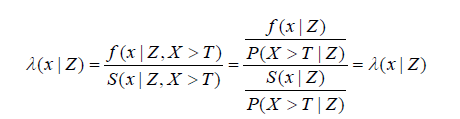
Additional conditioning on X > T is not required as all event times are within the observable region (X > T). Below, we explain why it is possible to consistently estimate ˆ β even if S(x) is not identifiable due to the presence of a RENO.
Assumptions necessary to establish the consistency of ˆ β are as follows:
1. (Ti,Yi,δi) are i.i.d for i ∈{1,·· ,n}
2. P(Yi ≥ Ti) > 0
3. Xi ⊥⊥ Ti.
4. Xi ⊥⊥ Ci
Given these assumptions, the likelihood of the observed duration Y conditional on the truncation time, T is:
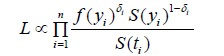
where f is the density function for the duration, S is the corresponding survival function, δi = I(xi ≤ ci), yi = min(xi,ci) and xi, ci, ti are observed duration, censoring and truncation times, respectively. Wang et al. [10] showed that the above likelihood can be factorized into the partial likelihood for β, LP(β) and a residual (ancillary) likelihood LR(β,λ0) that contributes no information for the estimation of β. The partial likelihood LP(β) is given by
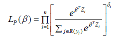
Where R(yi) is the risk set given by R(yi) =Pn j=1 I(tj ≤ yi ≤ yj). Estimators and large sample properties of β are derived based on LP(β). We let a⊗0 = 1,a⊗1 = a,a⊗2 = aaT and S(r)(β,x) = 1 nPn j=1 Qi(x)Z⊗r j eβT Zj where r = 0,1 and 2 and Qi(x) = I(ti ≤ x ≤ yi). Also, let v(β,x) be the limit of V (β,x) = S(2)(β,x) S(0)(β,x) −hS(2)(β,x) S(0)(β,x)i⊗2 and s(r)(β,x) be the limit of S(r)(β,x). Now let
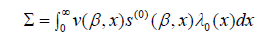
and assume Pis positive definite. Note this likelihood is similar to the usual right-censored data partial likelihood except for the diference in the definition of the risk set. Examining the form of the partial likelihood reveals that the presence of RENO wills not afect the estimation of β since no observations are made within it. Therefore, following argument from Andersen and Gill [11], ˆ β can be shown to be consistent. The regularity conditions and additional assumptions as stated in Andersen and Gill [11] are unafected bythe presence of RENO.
Summary of the Mochudi Relationship Data
The relationship dataset we consider arose from an AIDS prevention pilot study conducted in the village of Mochudi, Botswana. The dataset contains information on 2268 subjects who reported at least one relationship. For the 376 subjects who had two or more sexual relationships in our dataset, we consider only the most recent, which is defined as the partnership with the most recent sexual contact. We restrict the analysis of partnerships to relationship durations that are 10 years or less; longer relationship are censored at 10 years as the reliability of recall beyond 10 years is uncertain. Furthermore, for investigation of spread of STIs, it may be more useful to focus on relationships shorter than 10 years. There were 390 relationships that were greater than 10 years and only 8 (2%) of them had observed starting times. Therefore most of the information available for estimation of duration of relationships is from relationships that are shorter than 10 years. In total, we have 2050 (90%) ongoing (censored) relationships at the time of the survey interview. In addition, 992 (44%) partnerships are untruncated since they began within the sampling window of 12 months. Additional descriptive statistics pertaining to our population of study are provided in Tables 1 and 2.
| HIV Negative | HIV Positive | Combined | |
|---|---|---|---|
| N=1742 | N=502 | ||
| Age in years | (23,28,40) | (28,35,42) | (24,30,41) |
| Duration (X) in years | (.88,2,7) | (.99,3,7.99) | (.9,2,7) |
| Truncation (T) in years | (0,1,6) | (0,2,7) | (0,1,6) |
| Date of last sex** | (5,14,42) | (4,14,35) | (5,14,35) |
*Q1, Q2, Q3 refer to 25th, 50th and 75th percentiles, respectively.
**Refers to time (in days) from the last sexual contact to the interview date.
Table 1: Quartiles (Q1,Q2,Q3)8 of key covariates by HIV status.
Male |
Female |
|
|---|---|---|
N=790 |
N=1478 |
|
Age in years |
(24,31,43) |
(24,30,40) |
Duration (X) in years |
(.66,1.4,6) |
(.99,3,8) |
Truncation (T) in years |
(0,.48,5) |
(0,2,7) |
Date of last sex** |
(4,14,60) |
(5,14,31) |
*Q1, Q2, Q3 refer to 25th, 50th and 75th percentiles, respectively.
**Refers to time (in days) from the last sexual contact to the interview date.
Table 2: Quartiles (Q1,Q2,Q3)* of key covariates by gender.
Evaluating the quasi-independence assumption via Kendall’s Tau
Validity of the TPLE depends on the quasi-independence assumption, i.e. the independence of the truncation and duration variables within the observable region. This assumption allows for the factorization of the joint density of the failure time and truncation time within in the observable region [12]. If this assumption of quasi-independence is violated, the construction of the likelihood may not be valid and the estimates derived from it may be biased. Keiding and Moeschberger [13] showed that the nature of the bias in the product limit estimate depends on the correlation between truncation and event time. Unlike the independence assumption of censoring and failure times, it is possible to test for the independence of truncation and failure times nonparametrically [12,14]. This assumption can be tested within the observable region (i.e. the region where Xi ≥ Ti) since we have both pairs (Xi,Ti). The scatter plot of (Xi,Ti) show in figure 6 provides a graphical check of the independence assumption of the truncation and duration times within the observable region.

Figure 6: The observable region for the duration dataset.
We examined Kendall’s Tau statistic for the dependence of the duration and truncation variables and did not find evidence of association (Kendall’s Tau Statistic=-0.005, p-value=0.0003). Conditions under which duration and truncation variables can be dependent are briefly discussed in the appendix.
Illustration of RENOs in the Mochudi relationship dataset
Figure 7(a) displays the TPLE estimate of the distribution of most recent partnerships. Applying the steps identified in Section 3.1, we observe several ignorable RENOs of various sizes with the largest RENO being around 55 days wide. As discussed above, ignorable RENOs do not affect consistency of estimation of the distribution. Figure 7(a) shows that 50% of the most recent relationships are at least 6.75 years long. Figure 7(b) shows a significant difference in the distribution of partnership durations by gender (p-value<.0001); the median duration of relationships for women and men in Mochudi were 9.95 and 3.67 years, respectively.

Figure 7: (a) TPLE estimate of overall duration of duration of relationship (b) TPLE estimates of duration of relationship by gender; females (solid line) and males (dashed line).
Note that their partners did not need to reside in this village.
As discussed in prior sections, if the size of the sampling window w is less than the gap in the support of the truncation times we have a region in which consistent estimation of the distribution function for X is not possible. For the Mochudi relationship dataset w = 365 days, implying that intrinsic RENOs occur only if there is a gap that exceeds 365 days in the support of the truncation times or equivalently, the calendar time of relationship initiations. Examples of populations where such conditions might apply include those that experience mass circumcision campaigns that prevent young men from initiating relationships, or those where there is seasonal migration of young men due to work (i.e. farming, mining) [15,16] or those that are characterized by cultural or religious norms that prohibit relationship formation for a period of time. Conditions that would lead to initiation time gap of 365 days or more are unlikely for the community from which these data are sampled, though it may be plausible within age subgroups. Hence it is very unlikely that the consistency of estimation is compromised by the presence of RENOs.
Spline Modeling of Age Effect on Duration
We use penalized smoothing spline to model the effect of age on the duration of relationship controlling for HIV and concurrency status. Our analyses make use of the approach of Therneau and Grambsch [17] to characterize linear and nonlinear effects of age on relationship duration. The results, displayed in figures 8(a) and 8(c), show that the hazard of relationship termination decreases with age at relationship initiation among males. For this group, there is a significant linear effect of age at relationship initiation (p=0.0006) and no evidence of nonlinearity. However, for females (figure 8(c)), the hazard of relationship termination does not vary much across ages at relationship initiation. We found no significant linear (p=0.99) or nonlinear (p=0.24) effect of age at relationship initiation. We note that the people included in our sample do not come from a closed population; hence there is no constraint that these curves be consistent.

Figure 8: Spline regression modeling of the efect of age at start of sexual partnership on duration. Figures (a) and (c) show the impact of self-reported age at the start of partnership on the duration of the partnership for males and females, respectively. Figures (b) and (d) show the impact of partner-reported age at the start of partnership on the duration of the partnership for males and females, respectively. Dashed lines represent 95 % CI for Hazard Ratio while dotted lines represent where Hazard Ratio is equal to 1.
The effect of the partner-reported age of males (i.e. reported by females) on the duration of relationship is very different from the effect of self-reported age of males (compare figures 8(a) and 8(b)). There was a significant linear association with age at partnership initiation for self-reported, but not partner-reported, age. A similar discrepancy is observed when comparing self-reported vs partner-reported age in figures 8(c) and 8(d). Lastly, we note that whereas figures 8(a) and 8(d) look similar as we would expect, figures 8(b) and 8(c) do not, reflecting the fact that distribution of self-reported and partner-reported ages are similar for women but not for men.
This paper identifies the sampling condition necessary to obtain a consistent estimator distribution of partnership durations from retrospectively collected survey data: the partnership sampling window must be large enough to avoid potential gaps in the relationship formation times that may lead to regions where events are not observable. As shown analytically and via simulation, the presence of RENOs will lead to inconsistent estimation of the duration distribution function. Assuming a parametric form for the distribution of duration times does allow for consistent estimation of the distribution of durations even in the presence of intrinsic RENOs. However, misspecification of the parametric model can lead to biased estimation of the distribution of partnership durations [18]. Provided that truncation and duration times are independent within the observable region and that the size of the partnership sampling window is larger than the gaps in the truncation times, consistent estimators of the distribution of partnership duration are provided by either the standard TPLE or Lai and Ying’s version [9] of the TPLE. Conditional independence (given a covariate like age) also permits consistent estimation of duration distribution using TPLE. In the absence of such an assumption, consistent estimation is not possible.
This paper also addressed the impact of RENOs on estimation of covariate effects from a Cox proportional hazard model. The regression coefficients describing the effect of a covariate on the hazard of relationship termination can be consistent, even if consistent estimation of the distribution function is not possible, provided that the conditions described in section 5 and the references therein are satisfied. We described incorporation of covariate effects using spline models to investigate reported differences in relationship duration between men and women. Such gender differences have been noted in other populations as well [19,20] where women reported longer and more stable relationships.
Consistency of the TPLE estimator when there is RENO
We need to demonstrate
Stple(x)−S(x|x > τ8)| p → 0 (1)
sup x∈(x1,x2)|ˆ Stple(x)−S(x1)|p → 0 (2)
sup x∈(x2,x8)|ˆ Stple(x|X > x2)−S(x|X > x2)| p → 0 (3)
where x8 lies in the interior of the support of the duration distribution function F and the censoring distribution function G, and τ8 = inf{t : H(t) > 0} where H(t) is the distribution function for the truncation times. Now, recall that TPLE estimate of S(x) is
Stple(x) = Y yi≤x(1−di Ri)
where di =Pn j=1 I(yj = y(i)),Ri =Pn j=1 I(tj ≤ y(i) ≤ yj), and y(1),·· ,y(k) are distinct ordered observed failure times and t(1),·· ,t(k) are the corresponding truncation times.
Proof
Since there is no intrinsic RENO between [τ8,x1], claim (1) above follows directly from the results of [8] or [9]. In order to show claim (2), note that ˆ Stple(x),x1 ≤ x ≤ x2 can be factorized as follows:
ˆ Stple(x) = Qyi≤x1(1− di Ri )8Qx1<yi≤x(1− di Ri ) = ˆ Stple(x1)8 ˆ Stple(x) ˆ Stple(x1)
Since there are no observation made in the interval (x1,x), the TPLE puts a mass of zero and hence ˆ Stple(x1) = ˆ Stple(x) which proves claim (2).
Finally, claim (3) can be proven by factorizing ˆ Stple(x),∀x > x2 as follows :
ˆ Stple(x) = Qyi≤x1(1− di Ri )8Qx1≤yi≤x2(1− di Ri )8Qx2<yi≤x(1− di Ri ) = ˆ Stple(x1)8 ˆ Stple(x2) ˆ Stple(x1) 8 ˆ Stple(x) ˆ Stple(x2)
Since there are no observation made in the interval (x1,x2), the TPLE puts a mass of zero and hence ˆ tple(x1) = ˆ Stple(x2). Thus,
Stple(x) = ˆ Stple(x1)8 ˆ Stple(x) ˆ Stple(x2)
Now consider the TPLE estimator, ˆ S8(x), which is constructed based only on observations yi > x2. Note that this estimator can equivalently be represented as
S8(x) = Y x2<yi≤x (1−di Ri ) =ˆ Stple(x) ˆ Stple(x2)
where the second equality follows from the factorization of ˆ Stple(x) as shown above. Since ˆ S8(x) is a TPLE the results of [8] can be applied to show ˆ S8(x) uniformly converges to S(x|X > 2) i.e.
sup S8(x)− S(x) S(x2)|p → 0...................(1a)
Now observe that the only diference between ˆ S8(x) and ˆ Stple(x) is the presence of the extra term ˆ tple(x1) in the equation for ˆ Stple(x). Thus, we get
Stple(x) = ˆ Stple(x1)8 ˆ S8(x),∀x > x2.
Since ˆ Stple(x1) p → S(x1) an application of Slutsky’s theorem to (1a) leads to:
Sup x∈[τ8,x]|ˆ Stple(x)−S(x) S(x1) S(x2)|p → 0.
Lastly, observing ˆ Stple(x2) = ˆ Stple(x1), and once again applying Slutsky’s theorem to the above expression, we obtain the desired result:
Sup Stple(x|X > x2)−S(x|X > x2)|p → 0.
Conditions for dependence of duration and truncation variables
Because the Kendall’s Tau test did not find dependence between duration and truncation times, we first investigate one condition that can lead to dependence between the duration and truncation variables. This is indirectly accomplished by examining the implications of assuming independence between truncation and duration as described below.
First, let the sampling window, w, and interview date, τ, be fixed. Now, let us assume truncation and duration time are independent. Then we have:
T ⊥⊥ X ⇔τ −w−Tf ⊥⊥ Td −Tf ⇒−Tf ⊥⊥ Td −Tf (1)
where Tf and Td are relationship formation and dissolution times respectively. The last implication follows since w and τ are fixed. Since Td and Tf are random, it follows from (1)
−Tf ⊥⊥ Td −Tf ⇒ Td 6⊥⊥−Tf ⇔ Td ⊥⊥−Tf ⇒−Tf 6⊥⊥ Td −Tf (2)
To see why the last statement is true, note that if Td ⊥⊥ −Tf, we have Cov(−Tf,Td) = E[−TfTd] − E[−Tf]E[Td] = 0. Given this, we observe that Cov(−Tf,Td−Tf) = E[−Tf(Td−Tf)]−E[−Tf]E[Td−Tf] = E[−TfTd] + E[T2 f ] + E[Tf]E[Td]−E2[Tf] = E[T2 f ]−E2[Tf] = Var(−Tf) > 0. Since Cov(−Tf,Td −Tf) > 0 we know −Tf 6⊥⊥ Td −Tf which further implies T 6⊥⊥ X.
Thus, we have arrived at one condition in which the independence assumption of duration and truncation time can be violated; if the time of formation of the relationship, Tf, is independent of the time of the dissolution of the relationship, Td, then duration and truncation will be dependent.
In addition, if the sampling window w or the date of interview τ (or both) are random, we can examine the dependence between the duration (X) and truncation (T) variables by examining the covariance between them as follows:
Cov(T,X) = Cov(τ −w−Tf,X) = Cov(τ,X)−Cov(w,X)−Cov(Tf,X)
Based on the simple formulation above, the truncation and duration variable are dependent if the calendar time of interview, or the sampling window width or the formation time are associated with the duration reported. In other words, if there is a temporal variation in the reported durations (for example, if subjects that were interviewed recently reported longer durations) or if the size of sampling window was correlated to the duration of the partnership reported, we expect dependence between the truncation and duration variables. A recent study by Cornelisse et al. [21] suggests that there is a seasonal trend in the total number of partnerships reported; people report higher numbers of sexual partners in the three months before consultations in summer compared with winter. Although this study looked at the time trend in the number of partners reported it will be interesting to explore if the duration of partnerships also varied seasonally. In general, if there is dependence between the truncation time and duration of partnerships, the proper estimation of the distribution of duration should account for this dependence as discussed in Mackenzie [22] or Chaieb et al. [23].
This work was supported by grant from National Institute of Allergy and Infectious Diseases R3751164