Keywords
|
| community model architecture, data transmission time, data transmission cost, transmission overhead, data fusion filter, transmission impairment |
I. INTRODUCTION
|
| The architectural paradigms of data fusion are of prime importance as it physically implements the logical designs. There are many data fusion filter architectures available in literature namely, Thomopoulos Architecture, Distributed Blackboard Data Fusion Architecture, System-based Data Fusion Architecture, Hierarchical Data Fusion Architecture, Distributed Data Fusion Architecture and Decentralized Data Fusion Architecture. In this paper, a new architecture named community model architecture has been proposed. This paper also presents two algorithms to calculate Data Transmission Cost (DTC) and Data Transmission Overhead (DTO) based on the architecture as transmission cost is one of the prime factors related to transmission. The architectures available in literature does not ensure smooth transmission throughout filter levels irrespective of the environmental considerations. This paper compares the existing architectures in terms of different parameters like power consumption, fault tolerance etc. and shows that the proposed work decreases the total DTC and DTO when the number of nodes or local filter level increases. This is due to the fact that, it minimizes the impairments by referring to the reference sensor for each level of local filter and by transmitting them to the next level with zero or minimal impairments. Moreover, it was found that the formulation yields better result than the existing set of architectures. This paper is organized as follows - Section 2 introduces the classical data fusion architectures and their comparative study. Section 3 deals with the Community model architecture and incorporates two formulations regarding the calculations of the DTC and DTO. It also establishes two algorithms for DTC and DTO with respect to community model architecture. Section 4 deals with the comparative analysis based on the DTC and DTO. |
II. RELATED WORK
|
| The literature provides many architectural paradigms to induce data fusion [17]. It was found that the Thomopoulos Architecture, Distributed Blackboard Data Fusion Architecture, System-based Data Fusion Architecture, Hierarchical Data Fusion Architecture, Distributed Data Fusion Architecture and Decentralized Data Fusion Architecture give better result in different environments and their target applications. |
| A. Thomopoulos Architecture [2][3]: |
| Thomopoulos brought into light architecture for data fusion that consists of three modules, each of which integrates data at the different levels or modules in order to integrate the data namely - |
| Signal Level Fusion: Here the data correlation takes place through learning because there is no mathematical model to describe the phenomenon which is being measured. |
| Evidence Level Fusion: Here combination of data takes place at different levels of inference which is based on two factors namely statistical model and the assessment which the user requires in decision making or hypothesis testing. |
| Dynamics Level Fusion: Here the fusion of data is carried out using the existing mathematical model. |
| Thomopoulos emphasized that the three essential criteria to be considered by any data fusion system so as to achieve the desired performance are: |
| a) Monotonicity with respect to the fused information |
| b) Monotonicity with respect to the costs involved |
| c) Robustness with respect to any a-priori uncertainty |
| The other important factors are - channel errors, delay in data transmission etc. |
| B. Distributed Blackboard Data Fusion Architecture [3][4][9]: |
| In the Distributed Blackboard Data Fusion Architecture, the two sensors are connected to a number of transducers. These sensors in turn have a supervisor that controls the handling of conflicting sensor measurements from the available data. This is based on the confidence levels which are assigned to each sensor. The transducers help to acquire maximum possible information (with regards to temperature, pressure etc) from the physical system under analysis. The fusion algorithm gives a value which depends upon the data available to the two sensors. The supervisors assign confidence in the measurements to each of the sensor readings. Based on the confidence levels, the data are generated for the final selection of the output data set. |
| C. System-based Data Fusion Architecture [3][10][11]: |
| The System-based Data Fusion Architecture framework uses three vital steps to analyze a system namely identification, estimation and validation. |
| Identification: In this step, an inference about the system is drawn after interrogating the factors utilized in the data fusion process. Identification of the levels at which fusion must be carried out are found. Generally combination of data (if collected from similar sensors) can take place at the lowest levels of inference, while data collected from dissimilar sensors are always combined at higher levels. At first the redundancy in measurements and possible errors are checked. After identifying type of data (whether it is concentrated or sparse), determination of relevant method for its preprocessing is done. Then the inbuilt redundancy of the sensor system is measured. After that, true dimensionality is identified and the content is reduced without reducing the information content. |
| Estimation: In this step, estimation of the data is done at the relevant levels of inference. To select the data fusion algorithm, two appropriate taxonomies are used as mentioned: |
| a) A four level hierarchy that comprises of pixel, feature, symbol and signal levels is used. |
| b) At signal and pixel levels, data correlation takes place due to absence of any mathematical model to describe the measured phenomenon. |
| c) At the feature level, extraction of features is done from raw data which are combined thereafter. |
| d) At symbol level, combination of data is done using a mathematical model and analysis is done on the basis of logical and statistical inference. |
| Validation: At this very stage, confirmation of processed data and fused information is done where the following two procedures are implemented: |
| a) Performance assessment of the data fusion model is made by the measurement of uncertainty content (as in probability measure, classification of accuracy) in the solution. |
| b) Implementing a benchmark procedure for improvement of output results of data fusion model and thereby obtaining the most optimal techniques. |
| D. Hierarchical Data Fusion Architecture [7]: |
| In a hierarchical structure, the lowest level processing elements transmit information upwards, through successive levels, where the information is combined. The hierarchical approach to systems design has been employed in a number of data fusion systems and has resulted in a variety of useful algorithms for combining information at different levels of a hierarchical structure. General hierarchical Bayesian algorithms are based on the independent likelihood pool architectures or on the log-likelihood opinion pools. In this architecture, the focus is on hierarchical estimation and tracking algorithms. The ultimate reliance on some central processor or controlling level within the hierarchy means that reliability and flexibility are often compromised. Failure of this central unit leads to failure of the whole system. Changes in the system often mean changes in both the central unit and in all related sub-units. Further, the burden placed on the central unit in terms of combining information can often still be prohibitive and lead to an inability of the design methodology to be extended to incorporate an increasing number of sources of information. Finally, the inability of information sources to communicate, other than through some higher level in the hierarchy, eliminates the possibility of any synergy being developed between two or more complimentary sources of information and restricts the system designer to rigid predetermined combinations of information. The limitations imposed by a strict hierarchy have been widely recognized both in human information processing systems as well as in computer-based systems. |
| E. Distributed Data Fusion Architecture [5][6]: |
| The move to more distributed, autonomous, organizations is clear in many information processing systems. This is most often motivated by two main considerations; the desire to make the system more modular and flexible, and recognition that a centralized or hierarchical structure imposes unacceptable overheads on communication and central computation. The migration to distributed system organizations is most apparent in Artificial Intelligence (AI) application areas, where distributed AI has become a powerful tool. |
| F. Decentralized Data Fusion Architecture [5][8]: |
| A decentralized data fusion system consists of a network of sensor nodes, each with its own processing facility, which together do not require any central fusion or central communication facility. In such a system, fusion occurs locally at each node on the basis of local observations and the information communicated from neighboring nodes. At no point is there a common place where fusion or global decisions are made. A decentralized data fusion system is characterized by three constraints: |
| a) There is no single central fusion centre; no one node should be central to the successful operation of the network. |
| b) There is no common communication facility; nodes cannot broadcast results and communication must be kept on a strictly node-to-node basis. |
| c) Sensor nodes do not have any global knowledge of sensor network topology; nodes should only know about connections in their own neighborhood. |
| A decentralized organization differs from a distributed processing system in having no central processing or communication facilities. A decentralized data fusion system implemented with a broadcast, fully connected, communication architecture. Technically, a common communication facility violates decentralized data fusion constraints. However a broadcast medium is often a good model of real communication networks. A decentralized data fusion system implemented with a hybrid, broadcast and point-to-point, communication architecture. |
| G. Centralized Data Fusion Architecture [5][12][13]: |
| In centralized data fusion architectures, the fusion node usually resides in the central processor which receives information from all the sources of inputs from the environment. In this architecture, all the fusion processes take place in a central processor which uses the raw facts from the environmental sources. In this schema, the sources only obtain the observations as the measurement tool and transmit them to a centralized processor, where the data fusion process is performed physically. If the data alignment and data association are performed without having impairments then the required data transfer time is negligible and the scheme is supposed to be the optimized one. |
III. PROPOSED ARCHITECTURE – COMMUNITY MODEL ARCHITECTURE
|
| The proposed Community Model Architecture (Fig 1) uses n number of sensors to acquire data. |
| These data are then passed through different filter levels. After passing each filter level, the filtered data are verified from the reference sensor, which holds all the standard value for verification. If the filtered value matches with the data available through reference sensor then the data is simply propagated to the next level of filter for further filtration. Otherwise the data values are updated from the reference sensor. In this way, the data are propagated until it reaches the Master Fusion Filter (MFF) which fuses the received data from different filters. Thus, the adjacent and different filter levels can ease out the burden from MFF. The MFF uses multiple levels of filter for each sensor. These multiple filter levels have been used to refine the collected data from the sensors so that the fine tuning regarding the data can be done easily. As different filtering algorithms are executed at different filter levels, the necessity of fine tuned data increases at each of the associated levels. As it has a direct communication with the reference sensor to compare the fused data, the difference between the actual value and the transmitted value can be calculated. At each level, all parallel filters merge their individual sensor data with a common reference data and establishes a local system state after each level of filtration. After that these local estimates are sent to the parallel filters of the next level which repeats the same process until it reaches the Nth level of filtration. After traversing all the levels, the local estimates from the last level are finally fused in MFF to generate the global estimates. |
| The parallel filters have a common state vector as they all share common reference system. When the signals arrive to the filters at various levels, they are processed and transmitted. The MFF has to bear less burden here as the filters in each stage communicates with each other after referring the reference sensor and generate an intermediary local estimate state after each stage of filtration so that the local estimates in each stage can take a shape towards it's final global estimated shape. The estimations of each stage are transformed into a series of local estimates which finally transform itself into global estimated state. The MFF only receives the final Nth level of local estimates and then fuses the data that are required to produce the desired state of facts. When there are problems related to transmission, the signal can be dropped. To regenerate the desired signal, retransmission of such signals is required which causes significant overall delay as various delay will be incurred more than once as the entire will start from the beginning and it has to re-refer the reference sensor for the validity of the filtered data. |
| A. Related Terms: |
| The comparisons of different architectures require finding the Data Transmission Time (DTT) based on which the Data Transmission Cost (DTC) and Data Transmission Overhead (DTO) can be found. This section discusses about the terms related to the formulation of DTC and DTO: |
| (i) Perimeter (Pn) of a data fusion filter means the area through which the data is passed. The perimeter is an important factor related to data fusion as if the perimeter increases then more amounts of data can be filtered at a time. |
| (ii) Data fusion density (ρ) is a data fusion operator based on averaging that is weighted by the density of each particular data sample. If most of the generated data are fused by filters to calculate the local estimates then the data fusion density increases. |
| (iii) Flattening (F) is a measure of the compression of an object where the individual entries are collated to form the actual object. Data can be received either in the collated form or in the compressed form, to serve the fused local estimates. If it is true, the actual estimates can be measured otherwise it will lead to wring estimates. |
| (iv) Scale factor stability (S) is a measure of how good the gyro output is with respect to rotation input. It actually deals with the difference between the different angular inputs for a specific data set. As the signals can come from any direction, the required data set has to generate an output which helps to derive the local estimates with respect to the angular momentum. |
| (v) Alignment (A) represents data points that lie on a relatively straight path. The alignment has to be minimal to generate the estimated state and to derive the spectrum related to the fusion. |
| (vi) Random noise (NR) is a noise characterized by a large number of overlapping transient disturbances occurring at random. The random noise can be used to develop and determine the impairments based on which the transmission overheads are calculated as more and more inputted data and fused data are prone to noises due to the transmission path. |
| (vii) The uncertainty in the bias (H) of a parameter consists of the uncertainty due to drift, random variations and testing. |
| B. Mathematical Formulation: |
| This section deals with the formulation of DTC and DTO in terms of different parameters such as perimeter of a data fusion filter, data fusion density, flattening, scale factor stability, alignment, random noise, bias uncertainty etc. which have been discussed in the previous section. |
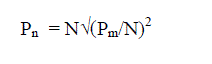
| Let N = Total number of local filters, Pm = Perimeter of master fusion filter, |
| Hence, Perimeter of each local filter(Pn) will be |
 eq. (1) eq. (1) |
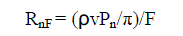
| If ρ= Data fusion density per LF, v=Average velocity of the light then the Crossing rate of different LF levels (Rn) is, |
 eq. (2) eq. (2) |
| Considering, flattening of the LF surface(F), the modified crossing rate is - |
 eq. (3) eq. (3) |
| If scale factor stability(S) is incorporated, equation (3) becomes, |
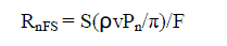 eq. (4) eq. (4) |
| Introducing random noise(NR), the formulation of crossing rate will be - |
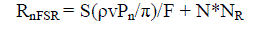 eq. (5) eq. (5) |
| Considering the alignment consideration as A, we get |
 eq. (6) eq. (6) |
| Taking the bias uncertainty(H) into account, |
 eq. (7) eq. (7) |
| If the latency time is LT then, |
 eq. (8) eq. (8) |
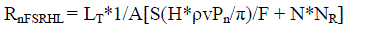
| So the transmission time up to Nth level will be the summation of the crossing rate of all the individual levels. And hence the DTT (TR) is - |
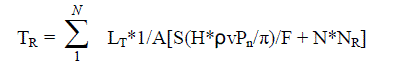 eq. (9) eq. (9) |
| If the power demand is PD and power generation is PG and the corresponding cost rate from filter level positions j to k as rjk, then the transmission cost [16] for each stage is - rjk*PD/(PG+PD). So the total transmission cost (CR ) is - |
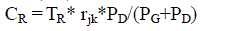 eq. (10) eq. (10) |
| If we assume that for M number of times the values has been updated from reference sensor then the transmission overhead [15] is - |
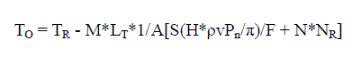 eq. (11) eq. (11) |
| C. Algorithm for Data Transmission Cost: |
| The Data Transmission Cost (DTC) procedure is one of the important steps related to the performance analysis of the community model. Here the DTC is to be determined based on the current scenario of the amount of data transmission and their corresponding data rate. Here the Data Transmission Time (DTT) [1] has been used, based on which the DTC procedure will be implemented. In this section, the algorithm for calculating the DTC has been discussed. Initially we input the standard parameter values [14] to the reference sensor so that they can be verified at a later stage. Initially the DTT is set to zero. Then the procedure Impairment Minimisation IM [1] is called and the values are initialised. If it is found that the data matches with the data already available with the reference sensor then it is calculated, otherwise they are updated and the total transmission time is calculated till the Nth level of filter is reached. After that the DTC is calculated from DTT based on the equation (10). Here TR denotes the total data transmission time and CR denotes the total data transmission cost. The DTC has been formulated as a function of data generation and data demand. The transmission cost for each pair of the filter levels has been chosen as rjk where r denotes their corresponding rate. For each filter level, the local estimates of cost are based on the transition and it is directly incorporated in the DTT. The community model algorithm is described in [1], for completeness the defined input parameters are denoted as the RS(i). |
| This (i) signifies the following - |
| A = Alignment consideration |
| S = Scale factor stability |
| H = Bias uncertainty |
| ρ = Data fusion density per local filter |
| V = Average velocity of the light |
| P = Perimeter of local filter |
| N = Number of filter level |
| Thus the explicit input parameters are RSA, RSS, RSH, RSρ , RSV, RSp, RSN. |
| Procedure: Data Transmission Cost |
| Step 1: Begin |
| Step 2: Input RSA, RSS, RSH, RSρ , RSV, RSp, RSN |
| Step 3: Set TR ← 0 |
| Step 4: Input LT, A, S, H, ρ, V, Pn, P, N, NR |
| Step 5: Call IM |
| Step 6: if (δ != Ø) || D !=RS |
| update A← RSA, S← RSS, H← RSH, ρ← RSρ, V← RSV, P← RSp, N← RSN |
| endif |
| Step 7: i ← 1 |
| Step 8: while (i <= N) |
| TR = TR + LT*1/A[S(H*ρvPn/π)/F + N*NR] |
| CR = CR + TR* rjk*PD/(PG+PD) |
| i ← i + 1 |
| end while |
| Step 9: End procedure |
| D. Algorithm for Transmission Overhead: |
| The Data Transmission Overhead (DTO) procedure is one of the important parameters to verify the performance of the community model architecture. Here the DTO is to be determined based on the current scenario of the amount of data transmission and their corresponding data rate. The DTO can be calculated based on the Data Transmission Time (DTT) [1] and will be implemented after the DTT procedure is completed. This algorithm describes the procedure to calculate the data transmission overhead. Initially we input the standard parameter values [14] to the reference sensor so that they can be verified at a later stage. Initially the DTT is set to zero. Then the values are inputted to the values to the procedure Impairment Minimisation (IM) [1]. If it is found that the data matches with the data already available with the reference sensor then it is calculated, otherwise they are updated and the total transmission time is calculated till the Nth level of filter is reached. After that the DTO is calculated from DTT based on the equation (11). Here TR denotes the total data transmission time and CR denotes the total data transmission cost. The DTO has been formulated as a function of data generation and data demand. After calculating the DTO if it is found to be simply a function of the IM then the number of iterations are calculated. If it is close to the number of filter levels then it is increased otherwise when it is close to zero the overhead decreases. The community model algorithm is described in [1], for completeness the defined input parameters are denoted as the RS(i). This (i) signifies the following - |
| A = Alignment consideration |
| S = Scale factor stability |
| H = Bias uncertainty |
| ρ = Data fusion density per local filter |
| V = Average velocity of the light |
| P = Perimeter of local filter |
| N = Number of filter level |
| Thus the explicit input parameters are RSA, RSS, RSH, RSρ , RSV, RSp, RSN. |
| Procedure: Data Transmission Overhead |
| Step 1: Begin |
| Step 2: Input RSA, RSS, RSH, RSρ , RSV, RSp, RSN. |
| Step 3: Set TR ← 0 |
| Step 4: Input LT, A, S, H, ρ, V, Pn, P, N, NR |
| Step 5: Call IM |
| Step 6: if (δ != Ø) || D !=RS |
| update A← RSA, S← RSS, H← RSH, ρ← RSρ, V← RSV, P← RSp, N← RSN |
| endif |
| Step 7: i ← 1 |
| Step 8: while (i <= N) |
| TR = TR + LT*1/A[S(H*ρvPn/π)/F + N*NR] |
| TO = TR - M*LT*1/A[S(H*ρvPn/π)/F + N*NR] |
| i ← i + 1 |
| end while |
| Step 9: End procedure |
IV. SIMULATION RESULTS
|
| Transmission Cost and Transmission Overhead are difficult steps in data fusion filtering. It consists of identifying and correlating noisy measurements, the genesis of which are unidentified because of several inescapable situations. The key models used in this fields are either deterministic (based on Classical Hypothesis), or probabilistic models (based on Bayesian Hypothesis). The values taken here as the standard parameters are bias uncertainty = 10 - 40, scale factor stability = 100-500, alignment = 200, random noise = 1 - 5, flattening = 1/298.257223563, latency time = 10 [14]. It is found that the proposed formulation of DTC in Community model architecture yields better result than that of Thomopoulos architecture, Distributed Blackboard architecture, System-based data fusion architecture, Hierarchical data fusion architecture, Distributed data fusion architecture, and Decentralized data fusion architecture. The DTC and DTO of each of these models has been calculated with the standard values using the respective formula and the result for level 1 are reflected in the following table . |
| The simulation studies involve the Community Model Architecture shown in Fig.1. The proposed algorithms – Data Transmission Cost and Data Transmission Overhead are implemented in MATLAB. The data are sent from source node 1 to destination node 8. The proposed algorithms are compared with the existing data fusion architectures like Thomopoulos Architecture, Distributed Blackboard Data Fusion Architecture, System-based Data Fusion Architecture, Hierarchical Data Fusion Architecture, Distributed Data Fusion Architecture and Decentralized Data Fusion Architecture. The results show that the metrics Data Transmission Time and Data Transmission Overhead are least in case of Community Model Architecture. |
| The architecture shown in Fig. 1 is able to transmit data upto nth level. Fig. 2 clearly shows that the metric Data Transmission Cost (DTC) is least in Community Model Architecture. In Fig. 3, the Data Transmission Overhead (DTO) is also least for Community Model Architecture as in both the cases, the required verification is done through the reference sensor for each of the filter levels. |
V. CONCLUSION
|
| This paper analyses signalling overhead, power consumption, fault tolerance, survivability and robustness facilities among different models and compares the community model architecture in terms of Data Transmission Cost (DTC) and Data Transmission Overhead (DTO). The community model architecture tries to reduce the transmission cost and overhead to improve the performance of data fusion in information processing. More over the transmitted data is much more accurate as they are compared with the reference sensor in each stage. The proposed architecture gives better result in terms of data transmission cost and data transmission overhead as the transmission time is less and the updating from reference sensor is required for less number of times. |
Tables at a glance
|
 |
|
| Table 1 |
Table 2 |
|
| |
Figures at a glance
|
 |
 |
 |
| Figure 1 |
Figure 2 |
Figure 3 |
|
| |
References
|
- B. Bhattacharya and B. Saha, “Community Model – A New Data Fusion Filter Paradigm” Sent in EAIT 2014.
- S. C. Thomopoulos, “Sensor Integration and Data Fusion”, Proceedings of SPIE 1198, Sensor fusion II: Human and machine strategies, pp.178–191, 1989.
- J. Esteban, A. Starr, R. Willetts, P. Hannah and P. Bryanston-Cross “A Review of data fusion models and architectures: towards engineering guidelines,” Journal Neural Computing and Applications Volume 14 Issue 4, pp. 273-281, December 2005.
- J. Schoess and G. Castore, “A distributed sensor architecture for advanced aerospace systems”, Proceedings of SPIE 932, Sensor Fusion, pp. 74-86, 1988.
- F. Castanedo, “A Review of Data Fusion Techniques”, The Scientific World Journal Volume 2013, Article ID 704504, 19 pages, 2013.
- M. E. Liggins, I. Kadar and V. Vannicola, “Distributed Fusion Architectures and Algorithms for Target Tracking”, Proceedings of the IEEE, Vol. 85, No. 1, pp. 95-107, January 1997.
- O. Kähler, J. Denzler and J. Triesch “Hierarchical Sensor Data Fusion by Probabilistic Cue Integration for Robust 3-D Object Tracking”
- H. Durrant-Whyte, “A Beginners Guide to Decentralised Data Fusion”, Australian Centre for Field Robotics, Version 1.0, pp. 1- 27, July 2000.
- P. K. Hou, X. Z. Shi and L. J. Lin “Generic blackboard based architecture for data fusion”, IECON 2000 (Volume 2), pp. 864-869, October 2000.
- R. Johansson “Information Acquisition in Data Fusion Systems,” TRITA-NA-0328 Licentiate Thesis Royal Institute of Technology Department of Numerical Analysis and Computer Science, Stockholm, Sweden, November 2003.
- W. Elmenreich, “A Review on System Architectures for Sensor Fusion Applications,” Lecture Notes in Computer Science, Springer, Vol. 4761, pp. 547-559, 2007.
- R. C. Luo, C. C. Chang and C. C. Lai “Multisensor Fusion and Integration: Theories, Applications, and its Perspectives” IEEE Sensors Journal, Vol. 11 No. 12, pp. 3122-3138, December 2011.
- E. F. Nakamura, A. A. F. Loureiro and A. C. Frery, “Information Fusion for Wireless Sensor Networks: Methods, Models, and Classifications,” ACM Computing Surveys, Vol. 39 No. 3, August 2007.
- C. R. Spitzer (Edited), “The Avionics Handbook,” CRC Press LLC, 2001.
- Y. Huang, J. P. Heritage, and B. Mukherjee “Connection Provisioning With Transmission Impairment Consideration in Optical WDM Networks With High-Speed Channels” IEEE Journal of Lightwave Technology, Vol. 23 No. 3, March 2005.
- A. J. Conejo, J. Contreras, D. A. Lima and A. Padilha-Feltrin, “ZbusTransmission Network Cost Allocation”, IEEE Transactions on Power ystems, Vol. 22, No. 1, February 2007.
- K. Kim, P. E. Pace, R. G. Hutchins and J. B. Michael, “A Comparison of Nonlinear Filers and Multi-Sensor Fusion for Tracking Boost- Phase Ballistic Missiles”, Naval Postgraduate School, Monterey, California, Center for Joint Services Electronic Warfare Technical Report (Prepared for U. S. Missile Defense Agency), January 2009.
|
BIOGRAPHY
|
| Boudhayan Bhattacharya is an assistant professor, Dept. of CA in Sabita Devi Education Trust – Brainware Group of Institutions. He received his M. Tech (CSE) degree from WBUT, Kolkata, India. His research interests are Data Fusion, Mobile Computing, NoC etc. |
| Dr. Banani Saha is an associate professor, Dept. of CSE in University of Calcutta. She received her Ph. D (Tech) degree from University of Calcutta, India. Her research interests are Data Mining, Data Warehousing, Image Processing, Data Fusion etc. |