1Department of Mathematical Sciences, University of Texas at Dallas, Richardson TX 75080, USA
2Department of Physics and Astronomy, Howard University, Washington, DC 20059, USA
Received date: 04/09/2015 Accepted date: 09/11/2015 Published date: 25/11/2015
Visit for more related articles at Research & Reviews: Journal of Statistics and Mathematical Sciences
We employ Mathematica to find ZN-invariant subgroups of E8 for application in M-theory. These ZN-invariant subgroups are phenomenologically important and in some cases they resemble the gauge groups of our real world. We present a specific example of ZN-invariant subgroups of E8, which turn up in orbifold compactification of M-theory. However, the procedure can be applied for any ZN group that acts by shifts (translations) in the root lattice of semisimple Lie groups with An, Bn, Cn, Dn, E6, E7 and E8 factors.
Orbifold compactification, String-theory, M-theory
In models where part of spacetime is compactified, the geometry of compact space affects the gauge symmetries of the model. Herein, we consider the Horava-Witten M-theory [1,2], where the 11th dimension is compactified to an interval, I, and there are two ten-dimensional planes at the boundaries of I. It is convenient to identify  , acting as
  , so that the boundary of I consists of the fixed points of this
  -action. On each one of these ten-dimensional spacetime planes there is an independent copy of E8 gauge fields (principal vector bundle). To produce considerably more realistic models with 4-dimensional spacetime, one may proceed as follows:
1. Impose twisted periodicity conditions on six of the ten dimensions of the boundary spacetime planes, passing  , where Λ is a suitable 6-dimensional lattice and Δ is a symmetry of Λ . We consider
2. Simultaneously embed the Δ action into the E8 structure group of the gauge fields on each of the two boundary spacetimes, the structure groups are broken to subgroups of E8 that are invariant with respect to the Δ-action.
This is referred to as “compactifying the Horava-Witten M-theory on a T6/Δ orbifold”, and Δ is the “orbifold group.” Typically, Δ acts by rotations on the compact space coordinates, and at the same time by shifts (translations) in the E8 root lattice [3,4].
In Ref [5], we have constructed  -orbifold models in M-theory. We used Mathematica to find the -invariant subgroups of E8. In this paper we present the details of the Mathematica computation codes and the procedure that we have used in Ref [5]. This procedure may be used, perhaps with minor adaptations, for higher order (iterated) orbifolds as well, and in situations where one needs to find the -invariant subgroups of any of the semisimple Lie groups with An, Bn, Cn, Dn, E6, E7 and E8 factors, where
  N acts by shifts in the root lattice.
Consider the root lattice  of one of the simple Lie algebras An, Bn, Cn, Dn, E6, E7 and E8. Let u denote a shift (translation) vector in acting as
  [3,4]; require moreover that (
 =1, so that u generates a N action on , and thus on G. The root vectors of g that are invariant with respect to this u-action
 (1)
(1)
are the root vectors of a subgroup HI ⊂ G that is invariant with respect to the N -action generated by u. Different shift vectors u define different N-actions, and therefore different N-invariant subgroups of G. Upon identifying those that are equivalent by G-conjugation, we find the inequivalent N-invariant subgroups, HI , for I = 1,2,… Without loss of generality, we restrict the  - valued components of u inshift to the standard range
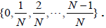
Note: As the so-defined N-invariant subgroups HI ⊂ G are explicitly defined in terms of the root lattice of G, they are by definition regular [6-13]. In addition, the conditionshift is trivially satisfied for the zero-weight vectors pC ={0,0, ,0} corresponding to Cartan generators of G. Therefore,
 (2)
(2)
and all so-defined N-invariant regular subgroups of G also have maximal rank.
Step 1: Find the set of positive root vectors of G, denoted W.
Step 2: Based on the above restrictions, we construct all possible N shift vectors v.
Step 3: Find all the subgroups1 HI ⊂ G .
Step 4: For each one of the subgroups HI ⊂ G , define the following four variables:
t is the set of positive root vectors of HI ⊂ G ;
p : = |t| is total number of positive root vectors in HI ⊂ G ;
r : = rankl(HI ), defined as the rank of semisimple part of HI ⊂ G , i.e., without U (1)-factors; m is number of A1 factors, if any, in HI ⊂ G .
These three variables can be read off by looking at the subgroup HI and can be used as identifiers of the group. If these three variables do not suffice to identify HI ⊂ G unambiguously, define another variable:
m2 is the number of A2 factors in HI, if any.
If {p, r, m, m2} turns out not to suffice to identify HI ⊂ G unambiguously, we look for A3, A4. . . factors in HI, the numbers of which, m3, m4...,will be necessary to identify HI ⊂ G unambiguously.
Step 5: Pick the first u from Step 2.
Step 5a : Set t = φ. For all  , append wa into the set t.
Step 5b: Compute {p, r, m, …} of this t (see Section 5 for the procedure).
Step 5c: Identify the subgroup HI ⊂ G by comparing {p, r, m, …} with the list from Step 4.
Step 6: Pick the next from Step 2, and go to Step 5a.
Steps 1–4 are preparatory. In particular, Step 4 sets up the string of identifiers {p, r, m, m2, …} as an “address” of the regular subgroups HI (I = 1, 2, 3, . . .) of a given simple Lie group G. For the purposes of specific applications, such as in M-theory [2,5,14] with G = E8 and N acting by translations in the root lattice (1), a subset of the identifiers {p, r, m, m2,…} sufficed.
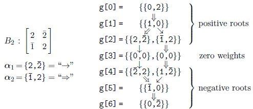
We take the adjoint representation of the group G and calculate its positive root vectors from the highest root using the standard algorithm [6,8-12]. Take for example the group G = E8. Any concrete representation of these roots will depend on a choice of a basis, and there exist at least three fairly standard conventions, corresponding to the labeling of nodes of the Dynkin diagram of E8, as shown3 in Figure 1. Being interested primarily in high energy physics applications such as in Ref [2,5,14], we follow the conventions of Refs [10,11], which provide the decades-long standard in the high energy physics.

Figure 1: The Dynk in diagram, the highest root of the adjoint representation and the Cartan matrix of E8, given in three fairly standard conventions and some corresponding references.
The highest root of the irreducible (248-dimensional) adjoint representation of E8 is {0, 0, 0, 0, 0, 0, 1, 0 }. The entire root system can be obtained from the highest root by subtracting from it the positive simple root vectors as follows: in any given root vector w, a positive value of the nth component, w[n], indicates the number of times the nth positive simple root αn can be subtracted from w minus the number of times αn can be added to w so as to get another root or zero [10,12]. For example, α1= {2,1, 0, 0, 0, 0, 0, 0} is the first positive simple root (and the 1st row in the Cartan matrix; Figure 1); it may be subtracted from itself twice4, producing: (3.1)
(3.1)
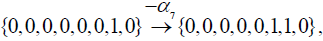
All three of these vectors are indeed in the root system of E8. Starting with λ = {0,0,0,0,0,0,1,0} , the positive simple root α7 ={0,0,0,0,0,1,2,0} may be subtracted once (since λ is the highest root, no positive root can be added and still get a root):
 (3.2)
(3.2)
Where upon 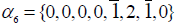 may be subtracted once
 (3.3)
(3.3)
Proceeding in this way halts with 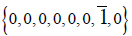 , having produced 240 (nonzero) root vectors and eight copies of {0,0,0,0,0,0,0,0} . Jointly, they span the 248-dimensional adjoint representation of E8.
In fact, every finite-dimensional unitary representation of any semisimple Lie group may be represented in a similar way: We recall that all such representations are spanned by weight vectors that are determined by a highest weight from which all others are obtained by iteratively subtracting the positive simple roots as outlined above; see Refs.[1-12]. By definition of λ being the highest weight, no positive simple root may be added to it and get a vector within the weight system of λ. Therefore, a positive nth component λ [n] >0 in the highest weight λ necessarily means that αn may be subtracted λ [n] >0 number of times from λ; plot the so-obtained “αn-descendants of λ,” (λ−kαn), k levels below λ. Now precede downward level by level, seeking an mth nth positive component in an αn-descendant weight of λ, from which to construct αm-decendants. Starting from a level where the mth≠ nth component (λ−kαn)[m] >0 but (λ−kαn+αm) is not in the weight-system (immediately above (λ−kαn)) implies that αm can be subtracted from (λ−kαn) precisely (λ−kαn) [m] number of times, αm-descendants.
Proceeding in this fashion eventually terminates and generates the complete weight system when starting from highest weights λ that define finite-dimensional representations [7,8,10-12]. Of course, one can just as easily start from the lowest weight and add the positive simple roots in the analogous fashion. In the special case of the adjoint representation, which is our focus at present, the nonzero weight vectors are called root vectors instead.
By plotting the weights (roots) below those from which they are obtained by subtracting positive simple roots and connecting them by arrows (for illustration, see (3.6) below), we obtain a “spindle shaped” graph called the weight (root) diagram of the (adjoint) representation. In the root diagram of the adjoint representation of a group G of rank r, the middle row of the root diagram is populated by r copies of {0,...,0}, representing the r Cartan generators. The row immediately above the middle is populated by the r positive simple root vectors; the roots above the middle row are the positive root vectors of G, while the roots below the middle row are the negative root vectors and are the sign-reversed copies of the positive root vectors. For every Lie group and its algebra, it therefore suffices to map out the subsystem of positive roots.
E8: The following Mathematica code computes the 120 positive root vectors of E8 following the conventions of Ref [10,11]. The code is adapted to any other convention by changing the basis for both the Cartan matrix and the highest root, i.e., the Mathematica variables a and g [0], respectively; for those displayed in Figure 1, a simple permutation of columns and rows will suffice. Also, we use “external/global” variable arrays so that the intermediate computations are all accessible, e.g., for troubleshooting and for tracing the functioning of the code; it is then necessary to start with clearing the required symbols, listed explicitly for each code. The Reader may also find the global command ClearAll ["Global‘*"] useful, which clears all user-defined variables from previous computations.
Input (1)
ClearAll [a, g, e];
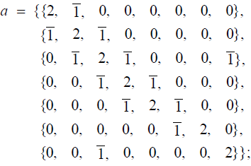
g [0] = {{0, 0, 0, 0, 0, 0, 1, 0}};
g [1] = Table[ Flatten[g[0]]- a[[Flatten[Position[Flatten[g[0]], 1]][[p]]]],
{p, Length[Flatten[Position[Flatten[g[0]], 1]]]}];
e[x_] : = e[x] = Union[Flatten[{Table[ Table[If[g[x][[j]][[i]] = = 1, g[x][[j]]- a[[i]],
If[g[x][[j]][[i]] = = 2, g[x][[j]]- a[[i]]]], {i, 8}], {j, Length[g[x]]}],
Table[Table[ If[g[x- 1][[l]][[k]] = = 2, g[x- 1][[l]]- 2 a[[k]]], {k, 8}],
{l, Length[g[x- 1]]}]}, 2]];
g[x_] : = g[x] = If[MemberQ[e[x- 1], Null], Delete[e[x- 1], 1], e[x- 1]];
Flatten[Table[g[m], {m, 0, 28}], 1])
Output (1)
Replacing Flatten [Table[g[m], {m,0,28}], 1] → Do[Print[g[m]], {m,0,58}] in the last line of input (1) prints all the roots, at their actual level and produces the characteristic spindle-shaped listing.
E7: For E7 and E6 the input codes are similar. For E7, the highest root of the adjoint representation, 133, is {1,0,0,0,0,0,0}. Its (133−7)/2 = 63 positive root vectors of E7 are found by the following code:
Input (2)
ClearAll [a, e, g];
g[0] = {{1, 0, 0, 0, 0, 0, 0}};
g[1] = Table[ Flatten[g[0]]- a[[Flatten[Position[Flatten[g[0]], 1]][[p]]]],
{p, Length[Flatten[Position[Flatten[g[0]], 1]]]}];
e[x_] : = e[x] = Union[Flatten[{Table[ Table[If[g[x][[j]][[i]] = = 1, g[x][[j]]- a[[i]],
If[g[x][[j]][[i]] = = 2, g[x][[j]]- a[[i]]]], {i, 7}], {j, Length[g[x]]}],
Table[Table[ If[g[x- 1][[l]][[k]] = = 2, g[x- 1][[l]]- 2 a[[k]]], {k, 7}],
{l, Length[g[x- 1]]}]}, 2]];
g[x_] : = g[x] = If[MemberQ[e[x- 1], Null], Delete[e[x- 1], 1], e[x- 1]];
Flatten[Table[g[m], {m, 0, 16}], 1])
E6: For E6, the highest root (weight of the adjoint representation), 78 is {0,0,0,0,0,1}. Its (78−6)/2 = 36 positive root vectors are found as follows:
Input (3)
ClearAll [a, e, g];
g[0] = {{0, 0, 0, 0, 0, 1}};
g[1] = Table[ Flatten[g[0]]- a[[Flatten[Position[Flatten[g[0]], 1]][[p]]]],
{p, Length[Flatten[Position[Flatten[g[0]], 1]]]}];
e[x_] : = e[x] = Union[Flatten[{Table[ Table[If[g[x][[j]][[i]] = = 1, g[x][[j]]- a[[i]],
If [g[x][[j]][[i]] = = 2, g[x][[j]]- a[[i]]]], {i, 6}], {j, Length[g[x]]}],
Table[Table[ If[g[x- 1][[l]][[k]] = = 2, g[x- 1][[l]]- 2 a[[k]]], {k, 6}],
{l, Length[g[x- 1]]}]}, 2]];
g[x_] : = g[x] = If[MemberQ[e[x- 1], Null], Delete[e[x- 1], 1], e[x- 1]];
Flatten[Table[g[m], {m, 0, 10}], 1])
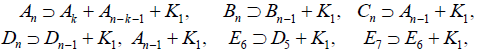
For the infinite sequences of Lie algebras An, Bn, Cn, Dn, we recall the low-dimensional isomorphisms [10]
C1 ≈ B1 ≈ A1, C2 ≈ B2, D2 ≈ A1⊕ A1, D3 ≈ A3. (3.4)
For this reason, we provide the Mathematica code below as follows: An for n > 1, Bn and Cn for n > 2,
Dn for n > 3, and provide the two remaining (low-n) cases explicitly, for illustration purposes:
 (3.5)
(3.5)
which correspond to the well-known  generators of SU2.
The Cartan matrix of C2 is the transpose of that of B2, so that the positive simple roots of C2 are the simply the swapped simple roots of B2, whereby the root system of C2 is identical as shown in (3.6).
An: For An, the dimension of the adjoint representation is n(n+2) and the number of positive root vectors is (n(n+2) − n)/2 = n(n−1)/2. The Mathematica code computing the positive root vectors of An, for n = 5 for example, is:
Input (4)
ClearAll [n, d, a, g, e];
n = 5; (* n = 2, 3, 4, ... *)
a = If[n > 1, Flatten[{{{PadLeft[d[[1]], n, 0, n- 3]}},
{Table[ PadLeft[ d[[3]], n, 0, n- i- 2], {i, n- 2}]},
{{PadRight[ d[[2]], n, 0, n- 3]}}}, 2], {2}];
g[0] = {RotateLeft[PadRight[{1, 1}, n, 0], 1]};
g[1] = Table[ Flatten[g[0]]- a[[Flatten[Position[Flatten[g[0]], 1]][[p]]]],
{p, Length[Flatten[Position[Flatten[g[0]], 1]]]}];
e[x_] : = e[x] = Union[Flatten[{Table[ Table[If[g[x][[j]][[i]] = = 1, g[x][[j]]- a[[i]],
If[g[x][[j]][[i]] = = 2, g[x][[j]]- a[[i]]]], {i, n}], {j, Length[g[x]]}],
Table[Table[ If[g[x- 1][[l]][[k]] = = 2, g[x- 1][[l]]- 2 a[[k]]], {k, n}],
{l, Length[g[x- 1]]}]}, 2]];
g[x_] : = g[x] = If[MemberQ[e[x- 1], Null], Delete[e[x- 1], 1], e[x- 1]];
Flatten[Table[g[m], {m, 0, n-1}], 1])
Bn: For Bn, the dimension of the adjoint representation is n(2n+1) and the number of positive root vectors is (n(2n + 1) − n) / 2 = n2 . The Mathematica code computing the positive root vectors of Bn, for n = 5 for example, is:
Input (5)
ClearAll [n, d, a, g, e];
n = 5; (* n = 3, 4, 5, ... *)
a = Flatten[{{{PadLeft[d[[1]], n, 0, n- 3]}},
{Table[ PadLeft[d[[4]], n, 0, n- i- 2], {i, n- 3}]},
{{PadRight[ d[[2]], n, 0, n- 3]}}, {{PadRight[d[[3]], n, 0, n- 3]}}}, 2];
g[0] = {PadRight[{0, 1, 0}, n, 0]};
g[1] = {Flatten[g[0]]- a[[Flatten[Position[Flatten[g[0]], 1]][[1]]]]};
e[x_] : = e[x] = Union[Flatten[{Table[ Table[If[g[x][[j]][[i]] = = 1, g[x][[j]]- a[[i]],
If[g[x][[j]][[i]] = = 2, g[x][[j]]- a[[i]]]], {i, n}], {j, Length[g[x]]}],
Table[Table[ If[g[x- 1][[l]][[k]] = = 2, g[x- 1][[l]]- 2 a[[k]]], {k, n}],
{l, Length[g[x- 1]]}]}, 2]];
g[x_] : = g[x] = If[MemberQ[e[x- 1], Null], Delete[e[x- 1], 1], e[x- 1]];
Flatten[Table[g[m], {m, 0, 2n-2}], 1])
Cn: Similarly to Bn, the dimension of the adjoint representation of Cn is also n(2n+1) and the number of positive root vectors is also (n(2n + 1) − n) / 2 = n2 . The Mathematica code computing the positive root vectors of Cn, for n = 5 for example, is:
Input (6)
ClearAll [n, d, a, g, e];
n = 5; (* n = 3, 4, 5, ... *)
a = Transpose[Flatten[{{{PadLeft[d[[1]], n, 0, n- 3]}},
{Table[PadLeft[d[[4]], n, 0,n- i- 2], {i, n- 3}]},
{{PadRight[d[[2]], n, 0, n- 3]}}, {{PadRight[d[[3]], n, 0, n- 3]}}}, 2]];
g[0] = {PadRight[{2}, n, 0]};
g[1] = {Flatten[g[0]]- a[[Flatten[Position[Flatten[g[0]], 2]][[1]]]]};
e[x_] : = e[x] = Union[Flatten[{Table[Table[If[g[x][[j]][[i]] = = 1, g[x][[j]]- a[[i]],
If[g[x][[j]][[i]] = = 2, g[x][[j]]- a[[i]]]], {i, n}], {j, Length[g[x]]}],
Table[Table[If[g[x- 1][[l]][[k]] = = 2, g[x- 1][[l]]- 2 a[[k]]], {k, n}],
{l, Length[g[x- 1]]}]}, 2]];
g[x_] : = g[x] = Delete[e[x- 1], 1];
Flatten[Table[g[m], {m, 0, 2n-2}], 1]
Dn: For Dn,0020 the dimension of the adjoint representation is n(2n−1) and the number of positive root vectors is (n(2n −1) − n) / 2 = n(n −1) . The Mathematica code computing the positive root vectors of Dn, for n = 5 for example, is:
Input (7)
ClearAll [n, d, a, g, e];
n = 5; (* n = 4, 5, 6, ... *)
a = Flatten[{{{PadLeft[d[[1]], n, 0, n- 4]}},
{Table[PadLeft[d[[5]], n, 0, n- i- 3], {i, n- 4}]},
{{PadRight[d[[2]], n, 0, n- 4]}}, {{PadRight[d[[3]], n, 0, n- 4]}},
{{PadRight[d[[4]], n, 0, n- 4]}}}, 2];
g[0] = {PadRight[{0, 1, 0}, n, 0]};
g[1] = Table[ Flatten[g[0]]- a[[Flatten[Position[Flatten[g[0]], 1]][[p]]]],
{p, Length[Flatten[Position[Flatten[g[0]], 1]]]}];
e[x_] : = e[x] = Union[Flatten[{Table[ Table[If[g[x][[j]][[i]] = = 1, g[x][[j]]- a[[i]],
If[g[x][[j]][[i]] = = 2, g[x][[j]]- a[[i]]]], {i, n}], {j, Length[g[x]]}],
Table[Table[ If[g[x- 1][[l]][[k]] = = 2, g[x- 1][[l]]- 2 a[[k]]], {k, n}],
{l, Length[g[x- 1]]}]}, 2]];
g[x_] : = g[x] = If[MemberQ[e[x- 1], Null], Delete[e[x- 1], 1], e[x- 1]];
Flatten[Table[g[m], {m, 0, 2n-4}], 1])
As with the E8 code Input (1), replacing
Flatten [Table [g[m],{m,0,mmax }],1] Do [Print [g[m]], {m,0,2mmax +2}] ( 3.7)
In the last line of the codes Input (2)–(7), where mmax is the index limit as shown above, prints all the roots at their actual level, forming the characteristic spindle-shaped listing.
The highest root, the level of positive simple root vectors (i.e., the height of the tower of positive roots) and the dimension of the adjoint representation can be found in Table 8 of [11], while Table 9 of Ref [11] gives the positive root systems of a few low-rank simple Lie groups. We leave it to the diligent Reader to adapt the above Mathematica codes for the remaining simple Lie groups, G2 and F4
In constructing  orbifolds for superstring theory and its M-theory extension, the choices of the N shift vectors (representing the embedding in the gauge group) are restricted. For example, in M-theory, the shift vectors must satisfy a supersymmetry condition, while in string theory they satisfy an additional modular invariance condition; herein, we impose only the former.
We give an example of vectors. There are 428 eight-component vectors that may be constructed with the components taking values in the standard range. The supersymmetry restriction requires that the components of a N vector add up to an integer [14]. The following code produces all such “supersymmetric” -vectors. We have shown only a sample of the output. Note that in order to find all the possible vectors preserving supersymmetry, we need to consider all permutations of the components of each one of the vectors produced by this code; this is accomplished by applying the Mathematica function Permutations [list] to each -vector produced in Output (8), below.
The code under Input (8) proceeds as follows:
a: stores a list of standard (fractional) nonzero values for the components of the -vectors (2.1). For general N , replace the values with proper fractions  , for k =1, ..., N .
b: stores, for 2 ≤ i ≤ 7 , a list of i-tuples of possibly repeated component-values from a, sorted and with duplicate i-tuples removed. For a Lie group of rank r, let 2 ≤ i ≤ (r −1) .
def.: The list-function complete [list] appends the negative of the total sum of the list-components, reduced mod 1, i.e., it appends a (possibly 0) component that makes the total sum into an integer.
c: applies the list-function “complete[list]” throughout the list of i-tuples “b”, completing them into i-tuples with integral totals.
q: stores the i -tuples from “ c,” padded by zeros to form 8-vectors, with sorted components, removed duplicates and sorted as vectors. For a Lie group of rank r, replace PadRight [c [[i]], 8] → PadRight [c[[i]], r] .
To relax the supersymmetric condition for the total sum of the components of the N-vectors v to be integral, omit line “c,” and replace c → b in line “q”; the line defining the list-function complete [list] thus becomes unused and may also be omitted.
Input (8)
ClearAll[a, b, c, q]; (* Clear arrays from previous computations *)
a = {1/7,2/7,3/7,4/7,5/7,6/7};
b = Union[Sort/@ Flatten[Table[Tuples[a,i],{i,2,7}],1]];
complete[list_] : = Append[list, Mod[-Total[list], 1]];
c = complete/@ b;
q = Sort[Union[Sort /@ Table[PadRight[c[[i]], 8], {i, 1, Length[c]}]]];
"Total no. of Z7 Vectors"
Length[q]
Output (8)
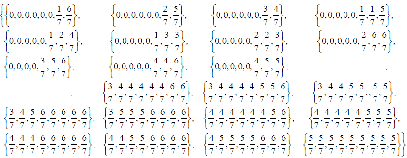
"Total No. of Z7 Vectors" 428
One may use a similar code for generating general N shift vectors in the root lattice for N≠7.
Our next step is to find all the regular, maximal-rank subgroups of G, using (2.1)–(2.2).
Our task is indeed closely related to the well-known problem of finding the regular subalgebras of the Lie algebra of G, which is accomplished by using the extended Dynkin diagram technique [6]; see also Refs [10-12]. The procedure starts with removing in every possible way one node from the extended Dynkin diagram of the Lie algebra of the original group G, producing a collection of Dynkin diagrams of the first list of maximal regular subalgebras. One then iterates this procedure for every Lie algebra from this first list. While this procedure is not perfect, all of the very few required corrections are known by now [12]
Many of the subalgebras are also found by the quicker method of removing from the extended Dynkin diagram of the group G several nodes in all possible ways at once, and reading off the subalgebra represented by the remainder. For example (Figure 2), if we take out the nodes α1, α6 and α7 from the extended Dynkin diagram of E8, we get D5 + A1; see Figure 2. Notably, however, this does not produce all subalgebras, such as for example  , which is obtained by the above-outlined iterative method, as shown in Figure 3. The resulting complete list of regular subalgebras of E8 has been known since Ref [6].

Figure 2: Removing the nodes α1, α6 and α7 from the extended Dynkin diagram of E8 gives the regular subalgebra D5+A1. “α+” denotes the extending node; “ × ” denote the locations of the removed nodes.

Figure 3: Removing the node α1 from the extended Dynkin diagram of E8 (top left) gives the maximal regular subalgebra D8 (top right). Removing the node α4 from the extended Dynkin diagram of D8 (bottom left) gives the regular subalgebra 2D4 ⊂ D8 ⊂ E8 (bottom right).
We then pass to the corresponding compact Lie (sub)groups. Rather importantly, the N-invariant regular subgroups are necessarily of maximal rank and include rank  abelian factors U1 , where HI is the semisimple factor of the N-invariant regular subgroup
  . This fact renders the centralizer of the semisimple factor in each N-invariant subgroup trivial, and effectively removes the distinction between inequivalently embedded subgroups; see Appendix 8 for details. The resulting list of maximal-rank regular subgroups of E8 is given in Table 1.
| Subgroups | p | m | r | c | |
|---|---|---|---|---|---|
| 0 | E8 | 120 | 0 | 8 | |
| 1 | SO16 | 56 | 0 | 8 | |
| 2 | SU9 | 36 | 0 | 8 | |
| 3 | SU8× SU2 | 29 | 1 | 8 | |
| 4 | SU6× SU3× SU2 | 19 | 1 | 8 | |
| 5 | SU52 | 20 | 0 | 8 | |
| 6 | SO10× SU4 | 26 | 0 | 8 | |
| 7 | E6× SU3 | 39 | 0 | 8 | |
| 8 | E7× SU2 | 64 | 1 | 8 | |
| 9 | SO12× SU22 | 32 | 2 | 8 | |
| 10 | SO8× SU24 | 16 | 4 | 8 | âÃÅÃâ |
| 11 | SU28 | 8 | 8 | 8 | |
| 12 | SU42× SU22 | 14 | 2 | 8 | âÃÅÃâ |
| 13 | SO82 | 24 | 0 | 8 | |
| 14 | SU34 | 12 | 0 | 8 | |
| 15 | E7× U1 | 63 | 0 | 7 | âÃÅÃâ |
| 16 | SO14× U1 | 42 | 0 | 7 | âÃÅÃâ |
| 17 | E6× SU2× U1 | 37 | 1 | 7 | âÃÅÃâ |
| 18 | SO12× SU2× U1 | 31 | 1 | 7 | |
| 19 | [SU8]‡ × U1 | 28 | 0 | 7 | âÃÅÃâ |
| 20 | SO10× SU3 × U1 | 23 | 0 | 7 | âÃÅÃâ |
| 21 | SO10× SU22× U1 | 22 | 2 | 7 | âÃÅÃâ |
| 22 | SU7× SU2× U1 | 22 | 1 | 7 | âÃÅÃâ |
| 23 | SO8× SU4× U1 | 18 | 0 | 7 | |
| 24 | SU6× SU3× U1 | 18 | 0 | 7 | |
| 25 | SU6× SU22× U1 | 17 | 2 | 7 | |
| 26 | SU5× SU4 × U1 | 16 | 0 | 7 | âÃÅÃâ |
| 27 | SO8× SU23× U1 | 15 | 3 | 7 | âÃÅÃâ |
| 28 | SU5 × SU3 × SU2× U1 | 14 | 1 | 7 | âÃÅÃâ |
| 29 | SU42× SU2× U1 | 13 | 1 | 7 | |
| 30 | SU4 × SU3× SU22× U1 | 11 | 2 | 7 | |
| 31 | SU33 × SU2× U1 | 10 | 1 | 7 | |
| 32 | SU4× SU24× U1 | 10 | 4 | 7 | |
| 33 | SU27× U1 | 7 | 7 | 7 | |
| 34 | E6× U12 | 36 | 0 | 6 | âÃÅÃâ |
| 35 | SO12× U12 | 30 | 0 | 6 | âÃÅÃâ |
| 36 | SU7 × U12 | 21 | 0 | 6 | âÃÅÃâ |
| 37 | SO10× SU2 × U12 | 21 | 1 | 6 | âÃÅÃâ |
| 38 | [SU6]‡ × SU2× U12 | 16 | 1 | 6 | âÃÅÃâ |
| 39 | SO8× SU3× U12 | 15 | 0 | 6 | âÃÅÃâ |
| 40 | SO8× SU22× U12 | 14 | 2 | 6 | âÃÅÃâ |
| 41 | SU5× SU3× U12 | 13 | 0 | 6 | |
| 42 | [SU42]‡ × U12 | 12 | 0 | 6 | |
| 43 | SU5 × SU22× U12 | 12 | 2 | 6 | |
| 44 |
SU4 × SU3 × SU2 × U12 |
10 | 1 | 6 | |
| 45 | SU33× U12 | 9 | 0 | 6 | |
| 46 | SU4 × SU23× U12 | 9 | 3 | 6 | |
| 47 | SU32× SU22× U12 | 8 | 2 | 6 | |
| 48 | SU3 × SU24× U12 | 7 | 4 | 6 | |
| 49 | SU26× U12 | 6 | 6 | 6 | |
| 50 | SO10× U13 | 20 | 0 | 5 | |
| 51 | SU6 × U13 | 15 | 0 | 5 | âÃÅÃâ |
| 52 | SO8× SU2× U13 | 13 | 1 | 5 | |
| 53 | SU5× SU2× U13 | 11 | 1 | 5 | |
| 54 | SU4 × SU3× U13 | 9 | 0 | 5 | |
| 55 | [SU4× SU22]‡ × U13 | 8 | 2 | 5 | |
| 56 | SU32× SU2× U13 | 7 | 1 | 5 | |
| 57 | SU3× SU23× U13 | 6 | 3 | 5 | |
| 58 | SU25 × U13 | 5 | 5 | 5 | |
| 59 | SO8× U14 | 12 | 0 | 4 | |
| 60 | SU5 × U14 | 10 | 0 | 4 | |
| 61 | SU4× SU2× U14 | 7 | 1 | 4 | |
| 62 | SU32× U14 | 6 | 0 | 4 | |
| 63 | SU3× SU22× U14 | 5 | 2 | 4 | |
| 64 | [SU24]‡ × U14 | 4 | 4 | 4 | |
| 65 | SU4× U15 | 6 | 0 | 3 | |
| 66 | SU3× SU2× U15 | 4 | 1 | 3 | |
| 67 | SU23× U15 | 3 | 3 | 3 | |
| 68 | SU3× U16 | 3 | 0 | 2 | |
| 69 | SU22× U16 | 2 | 2 | 2 | |
| 70 | SU2× U17 | 1 | 1 | 1 | |
| 71 | U18 | 0 | 0 | 0 |
Table 1. Regular subgroups of E8 and their identifiers described in the text. Double daggers (‡) indicates subgroups that have two inequivalent embeddings in E8 [6]. Whereas these are not distinguished by the identification of N -invariant subgroups described herein, their distinction is also made irrelevant by the inclusion of the U (1)8−r factors and by focusing exclusively on the adjoint representation; see Appendix A.
For this list of all maximal-rank regular subgroups of E8, we calculate the number of positive root vectors for each subgroup and list them in column p of Table 1. The values of the other identifiers (r, m and possibly m2, m3,…) turned out not to be necessary in most cases for our purposes5. Before using them, we found the possible candidates which are -invariant subgroups of E8 through a procedure given in Input/output (9). This greatly reduced the complexity of the codes in the next section and saves in the Mathematica evaluation time.
We have 428 7 shift vectors in Output (8) and once we take their permutations, this gives a total of 823, 542 shift vectors.
We take the first  vector from the previous section and calculate the number of positive root vectors that satisfy the condition p : v∈ using the following code:
Input (9)
p = (not shown here: 120 positive roots of E8 from Output());
v = Flatten[Table[Permutations[q[[i]]], {i, 1, 1}], 1];
u = Table[Table[p[[i]].v[[j]], {i, Length[p]}], {j, Length[v]}];
w = Table[ Table[IntegerQ[u[[j, i]]], {i, Length[p]}], {j, Length[v]}];
r = Table[Count[w[[j]], True], {j, Length[v]}];
Union[r] >>> Z7_Roots;)0pt
Output (9)
{37,42}
The code under Input (9) reads the 428 -vectors from Output (8) into the list “q” and the 120 positive roots from Output (1) into the list “p” and then proceeds as follows:
v: The list of -vectors v obtained as permutations of the first vector in Output (8).
u: Stores the dot products between each one of the vectors from “v” and the 120 positive roots in “p”.
w: Finds the integral dot products in “u”.
r: Counts the number of integral dot products in “u”, which is the total number of positive roots (in “p”) satisfying the condition p : v∈ , for each one of the vectors v in “v”.
The Output of this evaluation ({37,42}) is written in an external file Z7_Roots. We do this evaluation for the other vectors in Output (8) and the results are collected from the text file Z7_Roots. This gives the possible values of the identifier p for vectors as
P : {14, 15, 16, 21, 22, 23, 28, 30, 36, 37, 42, 63} (4.1)
This narrows down our choices to 21 subgroups of E8, marked by a check in column c of Table 1. Now we use the values of m (number of A1 factors in  ) to identify the possible subgroups . When p and m do not specify unambiguously, we use the values of r (rank of the semisimple part of HI). The values of the identifiers p, m and r are also calculated from the root vectors that are invariant (2.1) with respect to a shift. This is shown in the next section.
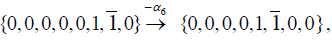
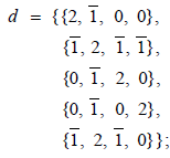
N Invariant Subgroups Of GTo illustrate the procedure of calculating the values of m and r from the -invariant root vectors we give the same example as in Section 3 of our previous paper [5]. Take the shift vector 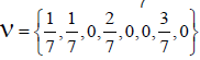 , which is one of the permutations of
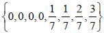 . The N-invariant E8 root vectors are
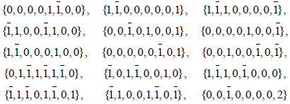 (5.1)
(5.1)
and are thus invariant under the action of the group generated by this shift. Call these root vectors t[i], i = 1, 2, …15, and set p = 15.
Next, we need to identify which subgroup -from among those listed in Table 1-do these roots (together with their negatives and the Cartan root vectors) generate. We look for possible relations in the form t[i] + t[j] = t[k] and find the following:
t[2]+t[14]= t[1], t[3]+t[13]= t[1], t[5]+t[9]= t[1], t[6]+t[8]= t[1], (5.2a)
t[3]+t[15]= t[2], t[5]+t[12]= t[2], t[7]+t[8]= t[2], (5.2b)
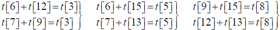 (5.2c)
t[7]+t[14]= t[6], t[12]+t[14]= t[9], t[14]+t[15]= t[13], (5.2d)
t[10]+t[11]= t[4]. (5.2e)
Since the root vectors t[7], t[10], t[11], t[12], t[14] and t[15] cannot be expressed as a sum of any other root vectors, they must correspond to 6 positive, simple root vectors in HI. The rank of the semisimple part of HI then must be 6, and the remaining two zero weights correspond to a U (1)2 factor. Also, all the 15 root vectors appear in (5.2), meaning this HI has no A1 factors, each of which would have had to have a single, isolated, positive root vector. From these -invariant root vectors the variables m and rare defined as:
m is the number of root vectors that do not appear in the equation of the form t[i] + t[j] = t[k] and so must be single, isolated, positive root vectors; here, m = 0.
r is the number of root vectors that do not appear on the right side of the relations of the form t[i] + t[j] = t[k] and so must be simple; here, r = 6.
Using {p, m, r} = {15, 0, 6}, we identify unambiguously the subgroup from Table 1, as SO8 × SU3. Observe that this is indeed consistent with the structure of the relations (5.2):
The positive roots t[4], t[10] and t[11] form a separate rank-2 positive root system where t[10] and t[11] are simple and t[4] is their sum (5.2e); this can correspond only to SU3.
The positive roots t[6], t[9] and t[13] are each obtained as a sum (5.2d) of two of the positive simple roots {t[7], t[12], t[14], t[15]}, and so must be one level above these positive simple roots.
Expressing t[6], t[9] and t[13] in this way, t[3], t[5] and t[8] are each found to be a sum (5.2c) of three of the positive simple roots, and so are two levels above the positive simple roots.
In this way, t[2] = t[7] + t[12] + t[14] + t[15] is a sum (5.2b) of all four distinct positive simple roots, while t[1] = t[2] + t[14] = t[7] + t[12] + 2 t[14] + t[15] has one more positive simple root (5.2a). Therefore, t[2] and t[1] occupy respectively the third and fourth level above the positive simple roots.
These facts are consistent with {t[7], t[12], t[14], t[15]; t[6], t[9], t[13]; t[3], t[5], t[8]; t[2]; t[1]} forming the positive root system of SO(8), i.e., its Lie algebra D4. As it turns out, such a more detailed study was not needed in determining the list of 7-invariant subgroups of E8 in Table 2 and the identifiers {p, m, r} did suffice to this end.
| Group | Group | Group | Group | ||||
|---|---|---|---|---|---|---|---|
| 1 | E7 | 5 | SO12 | 9 | SU8 | 13 | SU5× SU4 |
| 2 | E6× SU2 | 6 | SO10× SU3 | 10 | SU7× SU2 | 14 | SU5× SU3× SU2 |
| 3 | E6 | 7 | SO10× SU2 | 11 | SU7 | ||
| 4 | SO14 | 8 | SO8× SU3 | 12 | SU6× SU2 |
Table 2. -invariant subroups of E8
We employ this analysis in the construction of the Mathematica codes below and using the identifiers {p, m, r} identify the fourteen subgroups of E8 that are invariant under a shift listed in Table 2, and so in fact the complete group action generated by that shift.
Input (10)
q = (not shown here: 428 7 vectors from Output (8));
CleanSlate[]:
v = Flatten[Table[Permutations[q[[i]]], {i, 1, 1}], 1];
u = Table[Table[p[[i]].v[[j]], {i, Length[p]}], {j, Length[v]}];
w = Table[ Table[IntegerQ[u[[j, i]]], {i, Length[p]}], {j, Length[v]}];
s = Table[Flatten[Position[w[[k]], True]], {k, Length[w]}];
t = Table[ Table[p[[s[[j]][[i]]]], {i, Length[s[[j]]]}], {j, Length[w]}];
Φ [k_] : = Φ [k] = Evaluate[ b = Table[ Table[t[[k]][[i]] + t[[k]][[j]],
{i, Length[t[[k]]]}], {j, Length[t[[k]]]}];
c = Table[ Table[MemberQ[t[[k]], b[[i, j]]], {i, Length[t[[k]]]}], {j, Length[t[[k]]]}];
f = Position[c, True];
g = Union[Table[Sort[f[[i]]], {i, Length[f]}]];
x = Table[g[[i]][[1]], {i, Length[g]}];
y = Table[g[[i]][[2]], {i, Length[g]}];
h = Table[t[[k]][[x[[i]]]] + t[[k]][[y[[i]]]], {i, Length[x]}];
z = Flatten[Table[Position[t[[k]], h[[i]]], {i, Length[h]}]];
o = Table[l, {l, Length[t[[k]]]}];
m = Length[Complement[o, Union[x, y, z]]];
Table[If[Length[t[[k]]] = = 14, Evaluate[ Φ [k]; If[m = = 2, If[r = = 6, a[1] a[1] d[4],
If[r = = 8, a[1] a[1] a[3] a[3]]], a[1] a[2] a[4]]],
If[Length[t[[k]]] = = 15, Evaluate[ Φ [k]; If[m = = 0, If[r = = 5, a[5],
If[r = = 6, a[2] d[4]]], a[1] a[1] a[1] d[4]]],
If[Length[t[[k]]] = = 16, Evaluate[ Φ [k]; If[m = = 0, a[3] a[4], If[m = = 1, a[1] a[5],
If[m = = 4, a[1] a[1] a[1] a[1] d[4]]]]],
If[Length[t[[k]]] = = 21, Evaluate[ Φ [k]; If[m = = 0, a[6], a[1] d[5]]],
If[Length[t[[k]]] = = 22, Evaluate[ Φ [k]; If[m = = 1, a[1] a[6], a[1] a[1] d[5]]],
If[Length[t[[k]]] = = 23, a[2] d[5],
If[Length[t[[k]]] = = 28, a[7],
If[Length[t[[k]]] = = 30, d[6],
If[Length[t[[k]]] = = 36, Evaluate[ Φ [k]; If[r = = 6, e[6], a[8]]],
If[Length[t[[k]]] = = 37, a[1] e[6],
If[Length[t[[k]]] = = 42, d[7],
If[Length[t[[k]]] = = 63, e[7]]]]]]]]]]]]], {k, Length[t]}];
Union[%]>>>Z7_Groups;
Output (10)
{d [7], a[1]e[6]}
The code under Input (10) reads the 428 -vectors from Output (8) into the list “q” and the 120 positive roots from Output (1) into the list “p” and then proceeds as follows:
v, u, w: Have the same meaning as in Input (9).
s, t: For each one of the shift-vectors in “v”, these find the set of positive root vectors of E8 that have integral scalar products with the shift-vector.
Φ: This function uses the analysis as stated after equation (5.1) to find the values of m and r as defined in section 2. Note that Φ is a function which uses the variables “c”, “f”, “g”, “x”, “y”, “h”, “z” and “o” to evaluate “m” and “r” (which have the meaning of m and r from Section 2). This function is evaluated only when the number of -invariant roots of E8 (in the code this number is Length [t[[k]]]) is not enough to identify the subgroup HI as discussed in this section. The quantity Length [t[[k]]] is the number of -invariant root vectors ( = p), “m” is the number of A1 factors ( = m) and “r” is the rank (r) of a group. These three variables are calculated from the -invariant root vectors as explained in the above example, the 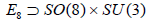 subgroup. The output of this evaluation is written in an external file Groups where a group An is identified as a[n], Dn as d[n] and En as e[n].
For other orbifolds there are situations where p, m and r do not suffice to specify the group unambiguously. In those cases we look for A2, A3, · · · factors in HI by looking at root vector relations. For example, an A2 factor would have to be spanned by three root vectors {t[i], t[j], t[k]} that satisfy an equation of the form t[i] + t[j] = t[k] and occur in no equation involving any other root vectors. Equivalently, we can look for root vectors that do not appear in any equation of the form t[i] + t[j] + t[k] = t[l].
Due to limitations of computer’s processor speed and memory, it may be necessary to partition the computation. The following shows how it may be done for the orbifold example in M-theory.
Collect all the vectors q in Output (8) and all the E8 root vectors p in Output (1) of section 3 and put them in a notebook, say, NB_0. Use the package ‘CleanSlate’6[14] and put this in one of Mathematica’s home directory ($HomeDirectory). This package helps in clearing the Mathematica kernel memory so that successive evaluations can use the maximum possible memory. The input of NB_0 are as follows:
Input (11)
q = ; (no output shown here: 428 vectors from Output (8) )
p = ; (no output shown here: 120 positive root vectors of E8 from Output (1) )
<< CleanSlate.m;
orbifold = EvaluationNotebook[];
NotebookSave [orbifold]
NotebookOpen ["NB_1.nb"])
(ii) We create a notebook Z7_Generic in $HomeDirectory which contains the code of Input (1) with some added lines of codes to make use of the automation process:
Input (12)
NotebookClose [orbifold]
CleanSlate[];
v = Flatten [Table[Permutations[q[[i]]], {i, α, α}], 1];
u = Table [Table[p[[i]].v[[j]], {i, Length[p]}], {j, Length[v]}];
w = Table [ Table[IntegerQ[u[[j, i]]], {i, Length[p]}], {j, Length[v]}]; r = Table[Count[w[[j]], True], {j, Length[v]}];
Union[r] >>> Z7_Roots;
orbifold = EvaluationNotebook[]; NotebookSave[orbifold]
γ = α + 1;
"NB " <> ToString[γ] <> ".nb";
InputForm [%]
NotebookOpen [%];
Next we create a notebook Z7_Generator with the following set of codes,
Input (13)
Do[NotebookPut[NotebookGet[First[Notebooks["Z7_Generic.nb"]]]/."α"->β];
NotebookSave[SelectedNotebook[],"NB "<>ToString[β]<>".nb"];
Pause [2]; NotebookClose [SelectedNotebook[]],β,1,428]
Once the Input (13) is run, it creates 428 notebooks with the contents of Input (12) where the value of
α = 1, 2, 3, · · ·, 428, respectively, for each notebook. The files are created in the $HomeDirectory.
(iii) Our next step is to evaluate these 428 notebooks in a way such that when we open NB_0, it au- tomatically evaluates it’s content and the contents of notebooks NB_1, NB_2 and so on so forth. The NotebookClose[orbifold] input line closes the previous notebook that has been evaluated. In this way the screen is not cluttered with open Mathematica notebooks, improving the performance of the computer’s memory. The memory is also managed by the input line CleanSlate[]. Note that the ‘CleanSlate’ package is called in after Mathematica stores the values of q and win its memory which is necessary for the whole evaluation process. The end result is collected from the text file Z7_Roots created in $HomeDirectory and is given in Eq. (4.1).
(iv) We apply a similar procedure for the evaluation of the 7
invariant groups, Input (10). The results are collected from the text file Z7 Groups and are summerized in Table 2.
In order for the automation process to work we need to make the following changes to Mathematica preferences,
1. Notebook Options → File Options → Notebook Autosave (False → True)
2. Notebook Options → File Options → ClosingAutosave (False → True)
3. Notebook Options → File Options → AutogeneratedPackage (Manual → None)
4. Notebook Options → Evaluation Options → Initialization CellEvaluation (Automatic →True)
5. Notebook Options → Evaluation Options → Initialization CellWarning (True → False)
6. Cell Options → Evaluation Options → Initialization Cell (False →True)
This automation process was first tested and used in version 5.2 of Mathematica, where it worked as designed. For later versions, there appears to be a problem which prevents the evaluation of a notebook when it is opened by another notebook, even though the Initialization CellEvaluation and Initialization.
Cell are changed to True (globally). In those versions of Mathematica, the automation process (iii) can be performed using a code such as:
Input (14)
nb = NotebookOpen ["notebook.nb"];
SelectionMove [nb, All, Notebook];
SelectionEvaluate [nb];
orbifold = EvaluationNotebook [];
NotebookSave [orbifold];
NotebookClose [orbifold];
Corresponding changes need to be made also in Input (11) and Input (12) for this automation process to work.
We have shown in detail how to find the -invariant subgroups of E8 using Mathematica. These groups, obtained in orbifold M-theory, turn out to be closely related to string theory compactification down to four dimensions: In the limit x11 → 0, the two - invariant subgroups of E8 (one on each of the two boundaries of x11) coalesce into  which turn out to coincide with the gauge groups found in -orbifold models in string theory [14]. We have tested our codes also for 2, 3, 4 and 6 orbifolds. The so-obtained subgroups upon the limit x11 →0 coincide with those found in string theory compactification. This would imply that our codes can also be used for 8 and 12 orbifolds.
In the presence of gauge background fields (Wilson lines) the four-dimensional gauge group breaks down to some smaller groups. Since these Wilson lines provide additional shifts in the group lattice, it should be possible to employ our procedure also in those types of models.
For the simple Lie groups An, Bn, Cn, Dn, E6 and E7, our procedure can be applied in finding the unbroken gauge symmetry under any N shifts. In section 3, we provided the root vectors for these groups. As semisimple Lie groups are products of simple Lie groups, the procedure merely needs to be applied to each factor separately.
Finally, our present goal was the demonstration that Mathematica can be used to compute Δ-invariant subgroups of semisimple Lie groups. Having been motivated by applications in M-theory, we have restricted ourselves to “supersymmetric” Δ-actions and to Δ = N for simplicity. Generalizations in both respect seem to be worthwhile, but are beyond our present scope. Similarly, it would seem desirable to re-structure and package the computations presented herein into a single, interactive Mathematica package, but that too is beyond our present scope.
Regular Subalgebras of E8
Physics applications in grand-unified model building [11] and string-theory and its M-theory extension [1,2] focus on compact classical Lie groups, and often also on an application-dependently restricted subset of their lowest-dimensional unitary representations. Such is the case in [1,5,14], where (1) only the adjoint representation of E8 is considered, and (2) only the N- invariant subgroups HI. In particular, the N-invariant subgroups HI ⊂ G all satisfy (2.1)–(2.2) and have a vanishing centralizer; see below. Also, finite factors and the real forms of the Lie groups are not considered and we easily pass from Lie algebras to the corresponding compact Lie groups.
A.1. Subalgebras
An exhaustive procedure for listing the regular subalgebras of Lie algebras was provided originally by EB Dynkin [6], is well described in texts [8,10,12], review literature [11] and also in research articles such as Ref [14]. One starts with listing the maximal semisimple regular subalgebras by removing one node from the extended Dynkin diagram of the original algebra. For E8, these are [6]:
 (A.1)
(A.1)
Next, proceed by listing the maximal semisimple regular subalgebras of (A.1), and continue so iteratively. This adds
 (A.2)
(A.2)
to the list (A.1), completing the list of all semisimple regular subalgebras of maximal rank [6, Table 10]. Non- semisimple maximal subalgebras are now found by applying to the list (A.1)–(A.2) the results in Dynkin’s Table 12.a [6]:
 (A.3)
(A.3)
Where  for n > 1 and
  and K1 is the “null algebra” consisting of a single certan element, generating an abelian factor U(1) in the corresponding Lie groups. For E8, this produces the listing
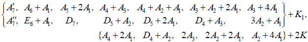 (A.4)
(A.4)
omitting the non-semisimple subalgebras wherein a K1 summand is subsumed within a proper A1 summand in an otherwise identical subalgebra in the listing. The two separate copies of A7 + K1 however are listed as inequivalent subalgebras, in that 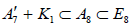 whereas
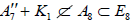 [6], which is easily traced in the progression from (A.1) to (A.2) to (A.4).
Finally, in addition to the combined listing of 8 + 6 + 19 subalgebras (A.1)–(A.2)–(A.4), the remaining 42 subalgebras are obtained by omitting summands from the entries (A.1)–(A.2)–(A.4) in all possible ways. In doing so, one must take into account that the omitted summands may turn out to be subsumed in the (larger) centralizer in E8, inducing an equivalence of the remaining summand(s). For example, already in the list (A.1) we have the evidently inequivalent rank-8 semisimple subalgebras A7+A1 and E7+A1.Omitting the larger summands, we obtain two subalgebras 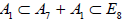 and
and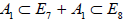 .However, it turns out that these two different embeddings are in fact equivalent by E8-conjugation [6], so that the centralizer of
  is always E7; this E7-centralizer subsumes the A7 from the former subalgebra chain.
In turn, omitting A1 from  leaves the rank-7 subalgebra
 with A1 the centralizer in E8. Since
 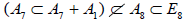 , the so-obtained subalgebra A7 cannot be isomorphic to
  in (A.4). This identifies
  as Dynkin’s in (A.4), since the first subalgebra pattern in A.3 and Dynkin’s distinction of imply that
It turns out that the remaining isomorphic but inequivalently embedded pairs of four subalgebras,
 (A.5)
(A.5)
are similarly distinguished by their (carefully traced) centralizers in E8. The resulting 76 proper subgroups corresponding to these algebras (including the  abelian factor corresponding to the Cartan subalgebra) are listed in Table 1.
A.2 Maximal-rank regular subgroups
The preservation by the N-actionshift of the abelian factor in  renders the centralizer of trivial.
To see this, consider for example the distinct maximal regular subalgebras  and
and  , where
  whereas
 [6].Omitting the 1 A summand from the latter results in two inequivalently embedded A7 subalgebras of E8 : the centralizer of
  is 0, while the centralizer of
  is A1 .
Passing to the corresponding compact Lie groups, we thus have the two inequivalently embedded SU8 subgroups of E8 , shown here paired with their respective centralizers:
 (A.6)
(A.6)
The N-invariant subgroups (2.1)-(2.2) of E8 that contains an SU8 factor is however  . In the case of
  , this , this N- invariant U1 factor is simply all of the centralizere (A.6). For
  however, the N-invariant U1 factor is a proper subgroup of the centralizer,
  , the centralizer of which is
  Therefore, we obtain that
 (A.7)
(A.7)
It then follows that the two N-invariant subgroups  , differing in the inequivalently embedded
  factors, nevertheless have the same (trivial) centralizer in E8. Finally, we are herein considering neither how the N -variant complement of the adjoint representation transforms with respect to the n -invariant subgroup HI nor how any other E8 -representations might transform under HI. This then leaves no way to distinguish the two copies of , which is why only one copy is listed in Table 1.
The situation is similar for the other four subgroups,  and only one copy of each of these is listed in Table 1.
It is gratifying to note that the complete listing of maximal-rank regular subgroups of E8 as given in Table 1 is also obtained by an iterative application of Tables 14 and 15 in Ref [11].
We should like to thank the Referee, for the superb work and constructive criticism in reviewing the initial version of this article, and for pointing out a serious error in some of the intermediate results. Although their correction turns out not to change the final result (Table 2), it did provide an opportunity not only to present our results correctly but also to better explain the details of the work and to clarify the subtleties in identifying the maximal-rank subgroups; see Appendix A. We are indebted to the generous support by the Department of Energy through the grant DE-FG02-94ER-40854. T.H. wishes to thank for the recurring hospitality and resources provided by the Physics Department of the University of Central Florida, Orlando, and the Physics Department of the Faculty of Natural Sciences of the University of Novi Sad, Serbia, where part of this work was completed.
1For all simple Lie groups of rank ≤ 8 and several of higher rank, the maximal subgroups are listed in the literature [6,11,13];
2Since the root lattice shift v corresponds to a generator g(v)∈N so that all elements of N are powers of g(v), it follows that root vectors satisfying v.wa = are in fact invariant with respect to all of N.
3To save space, negative root vector components are denoted by an over-bar: ¯1 d = ef −1, ¯2 d = ef −2, etc.
4To be meticulous, the fact that the first component of á1= {2, 1,0,0,0,0,0,0} is α1[1] = +2 merely means that we can subtract α1 from itself two more times than we can add α1 to itself, and still get a root or zero. However, since á1 + á1 ≠ 0 can be shown not to be a root, it follows that α1 can be added to itself zero number of times while staying in the root system, and so can be subtracted from itself precisely two times.
5The identifiers r and m are shown in Table 1 for completeness and for the benefit of possible generalizations to N-actions where the supersymmetry condition is relaxed. The additional identifiers, mi in Step 4, are easily added
6This package is available on-line at: http://library.wolfram.com/infocenter/MathSource/4718/.