Khalid Alnowibet1* and Lotfi Tadj2
1King Saud University, College of Science, Department of Statistics and Operations Research, Riyadh, Saudi Arabia
2Fairleigh Dickinson University, Silberman College of Business, Department of Information Systems and Decision Sciences, Canada
Received date: 23/07/2016; Accepted date: 24/08/2016; Published date: 27/08/2016
Visit for more related articles at Research & Reviews: Journal of Statistics and Mathematical Sciences
This paper analyzes an MX/G/1 queueing system where the server is subject to random breakdowns and the server applies the D-policy in providing the service. The steady-state queue size probability distribution is obtained using the embedded Markov chain technique. Key performance measures of the system are derived to obtain the optimal value of the threshold level D that minimizes the expected total cost per unit of time. The theoretical results are verified by special cases with published formulas.
MX/G/1 queue, Compound, Poisson process, Steady-state distribution, Breakdown, Fluctuation theory, Embedded Markov chain, D-policy
The single server queueing model with control policies has a wide range of applications in the quality control of telephone switching systems and production systems. As a result, several variations of the controlled queueing model have been studied extensively in the literature. These studies give rise to several types of control policies. To name a few, Yadin and Naor [1] analyzed the control policy in which the server doesn’t start service in idle period unless there are N customers in queue, which is called the N-policy. The T-policy is another control policy, introduced by Heyman [2] . The T-policy suggests turning the server into active state after a time interval of length T when the server is in the idle state. Later, the D-policy is proposed by Balachendran [3] which is the focus of this research. In the D-policy, the server remains inactive until a total of D service times are accumulated in the queue. Many variations of these control policies were suggested in the literature. A comprehensive survey paper in this topic is found in Crabill et al. [4] and Doshi [5,6] .
In this research, we derive the steady state distribution of a bulk-arrival queueing model with an unreliable single server under D-policy. In the queueing model under consideration, the server is switched to the inactive mode upon the completion of each busy period. Later, the server is switched to active mode when the total service times of all customers waiting in the queue exceed some pre-specified value D. Further, it is assumed that the server is subject to unpredictable breakdowns. The server is repaired immediately when a breakdown occurs and then put back into service.
The D-policy M/G/1 queueing system first introduced by Balachandran [3] , Balachandran and Tijms [7] , Gakis et al. [8] and many others in the literature, assume that the server has no breakdowns. Balachandran and Tijms proposed the optimal D-policy with reliable server using the expected number of customers in the system. Gakis et al. obtained the probability of busy server in the single server queue under D-policy. An approximation technique is proposed by Sivazlian [9] for obtaining the optimal D-policy used. Sivazlian approach uses the first three moments of the service time distribution to approximate the behavior of the system. In addition, Gakis et al. mathematically showed that the probability that the server is busy in the steady-state is equal to the traffic intensity. Li and Niu [10] analyzed a general GI/G/1 queue with D-policy to obtain the probability distribution of waiting customers in queue. An extension of a single server queue under D-policy is carried over by Rubin and Zhang [11] where they incorporate a setup time for switching on the service. Abolnikov and Dshalalow [12] used the first passage technique to the analysis of a number of stochastic models. Dshalalow [13,14] investigated the queue length of the system under a combination of N-policy and D-policy. Dshalalow proposed in his work an (N,D)-policy in which the server remains idle until the number of customers in queue is N or the total sum of service times for customers in queue exceeds D. Wang et al. [15,16] obtained the optimal D-policy using the expected length of the busy period, the idle period, and the breakdown period. Recently, Liu and Deng [17] examined a discrete-time D-policy Geo/G/1 queue with Bernoulli feedback and obtained the steady-state system size distribution using a decomposition method.
The bulk-arrival queues received a great attention by researchers since 1959 due to their wide applications. Gaver [18] seems to be the first to explicitly study bulk-arrival queues. Since then several models of bulk arrival queues evolved. Gross and Harris [19] provide a good survey for the uncontrolled bulk-arrival queues. For the controlled bulk-arrival queues, Yadin and Naor analyzed the bulk-arrival queue under the N-policy in which the server starts service if there are at least N customers in the queue. Dshalalow used the excess level processes to analyze bulk queueing systems in which N- and D-policies combined into one policy. Lee et al. [20] successfully combined the batch arrival queue with N-policy and obtained the analytical solutions. Later, Lee et al. [21] analyzed in detail the same system under N-policy with a single vacation. However, we noticed that the bulk-arrival queues with D-policy did not receive the same attention as the N-policy.
In practice, there are many situations where the D-policy is applied. Liu and Deng [17] presented the use of D-policy in a wireless local area network (WLAN). In WLAN, signals are received by the special access points and they are identified and transmitted if the access point is free. Otherwise, the received signals are placed in queue. Due to power saving, the access point is designed to serve exhaustively whenever the workload of signals reaches some level. Another practical example of this control policy is the mail handling system introduced by Wang et al. [16]. At the mail handling office, parcels are sorted into categories. The waiting line in the system is considered sorted. When the sorting process exceeds D units of time, the distribution machine is turned on and starts dispensing the parcels into slots according to the destination post office. It is expected that the machine may break down during the sorting process and it must immediately be repaired.
This paper is aimed to derive an explicit expression for the steady-state distribution of the number of customers in the queue. Using the steady-state distribution, conventional performance measures such as: expected length busy period, expected number in queue, expected waiting time, expected length of idle period, and probability that the server is busy all will be easily calculated. In addition, the steady-state distribution gives flexibility in obtaining nonconventional performance measures that may rise from the nature of the application. Another objective of the paper is to compute the optimal value of D-policy at which the minimum expected operation cost function is achieved.
In the model we consider, customers arrive to the system in batches of different sizes. The batches arrival is assumed to follow the Poisson process with a constant rate of λ>0. Thus, customers arrive according a compound Poisson process. The sizes of batches are discrete independent and identically distributed random variables X with a general distribution function that has a probability generating function a(Z) =E [Z X] and finite first two moments a1=E [X] and a2=E [X2] . Once the batch arrives to the system, customers in the batch enter the system and wait in single queue for service. Each customer in the system requests a single service and remains in the system until receiving his service.
The server provides service for each customer with random duration of service. The service times B of the customers are independent and identically distributed random variables having a general distribution function (CDF) B(t), Laplace-Stieltjes transform (LST) defined by B*(s)=E[e-sB], finite first moment b1 and finite second moment b2.
In this model, the server is subject to random sudden breakdowns. The rate at which failures occur on the server is assumed to be constant α >0 and failures follow a Poisson process. The repair of the server starts immediately when a failure occurs. Repair duration takes a random time R and the repair times are independent and identically distributed variables having a general CDF R(t), LST given by R*(s)=E[e-sB], finite first moment r1 and finite second moment r2.
To incorporate the breakdowns and repair times in our queueing model, we define a modified service time that integrates the actual service time with the possible repairs. We define the random variable G to be the modified service time which includes the service and possible repair times. The modified service time G has CDF G(t) and LST G*(s) = E[e-sG] with finite first and second moments g1 and g2, respectively. The modified service times are related to the actual service times and repair times through the following expression:
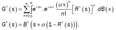 (1)
(1)
Using the equation (1), the first two moments of the modified service are given as follows:
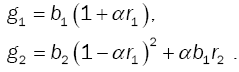 (2)
(2)
We, also, assume that the server applies first-come-first-served discipline under D-policy. At a service completion epoch, the server serves the next customer in line. Otherwise, if no customer is present in the queue after the last service completion, the server remains idle and waits for the workload to accumulate. While in the idle period, the service doesn't start the busy period until the total sum service times of the present customers are at least D units of time at the arrival of a customer.
We need to define the steady-state distribution for the number of customers in the system. Denote the queueing process Q(t) to be the number of customers in the system at time t ≥ 0. Consider the following random variables:
Q(t) : Number of customers in the system at time t;
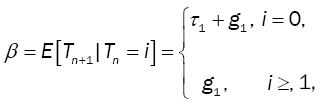
Tn : Completion epoch of nth service;
Qn : Number of customers in the system at a service completion epoch 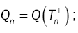
τn : Arrival time of nth group of customers, let τ0=0;
Xn : Size of the of nth group of customer, let X0=0;
Yn : Service time of nth customer, let Y0=0;
Bn : Cumulative service time, up to nth customer, 
Our approach is to derive the probability generating function (PGF) of the number of customers in the system that will be used to obtain the steady-state distribution of {Qn} using fluctuation theory. From Abolnikov and Dshalalow [12], we state the following theorem:
Theorem 1
For a single server queue under D-policy with compound Poisson arrival with rate λ > 0 where service times have LST B*(s), the random variables defined above have the following marginal distributions:
The index of the arriving customer causing the first excess of D, denoted by 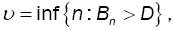 has the following marginal distribution:
Given that the projection of the first excess level Bυ on the process {An} where 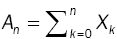 , the level of the first excess of D, denoted by Sυ, has the following marginal distribution:
The time at which the arriving batch of customers causes the first excess of D, denoted by τυ, has the following marginal distribution:
 (5)
(5)
The operator LD (âÃËÃâ¢) is defined as:
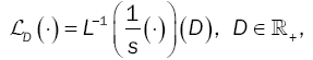
and L-1 is the inverse Laplace transform.
From the above theorem, we derive the PGF of the queueing process {Qn}. The process {Qn} is an embedded Markov chain with transitions defined as follows:
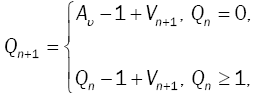 (6)
(6)
where Vn represents the number of customer arrivals during the th modified service time. Thus,
 (7)
(7)
Denote by A the transition probability matrix (TPM) of {Qn} and by Ai (z) the probability generating function of the ith row of A. Then,
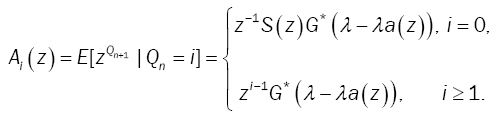 (8)
(8)
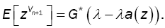
Note that the probability generating function of the index of the first excess is given by:
 (9)
(9)
Theorem 2
Le ρ = λg1where g1 represents the first moment of the modified service time. Then, the embedded process {Qn} is ergodic if and only if,
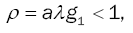 (10)
(10)
Where from (1)
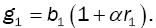 (11)
(11)
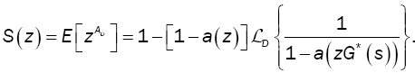
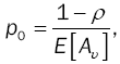
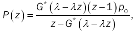
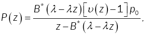
From Theorem 2, the steady-state probability distribution p of the TPM exists and, 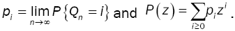 Then, from the relation
 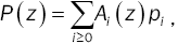 we have:
 (12)
(12)
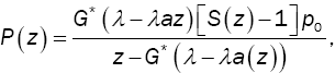
and the steady-state probability distribution is expressed in terms of the PGF P(z), where
 (13)
(13)
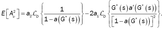
is derived from the initial condition P(1) = 1and E [Aυ ] is expressed as:
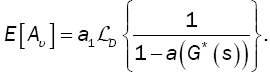 (14)
(14)
In this section we express mathematically some key performance measures that enable making decision to improve the behavior of the system.
Average Number of Customers (L)
In queueing theory, one of the main measures of performance is the average number of customers in the system (L). The value of this measure is obtained for our model by:
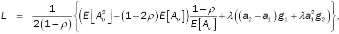 (15)
(15)
where g1 is given by (11) and  by (14), while g2 and
  are respectively given by
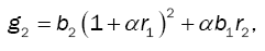 (16)
(16)
 (17)
(17)
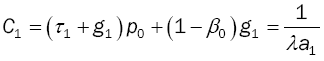
Service Cycle Distribution
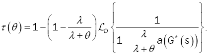
In practice, some systems encounter high cost of operation which makes the D-policy a good choice to control the system toward lower operation cost. Thus, the estimation of the length of continuous operation period is important to minimize the cost. The service cycle for a single server queueing system under D-policy with bulk arrivals and unreliable server is defined as the time interval between two consecutive customer departures, i.e., between two consecutive service completion times. In equilibrium, the random variable (C) of the service cycle has the LST expressed as follows:
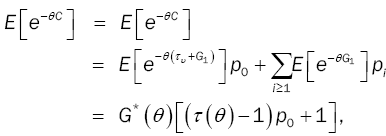 (18)
(18)
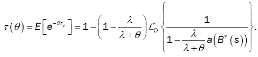
where the first passage time has LST
 (19)
(19)
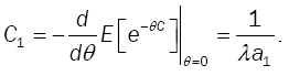
Mean Service Cycle
 (20)
(20)
The average service cycle in equilibrium is the negative derivative of LST in (17) at θ = 0. Then, the expected time between two service completion epochs in equilibrium is given by:
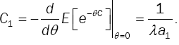
Another way to establish this result is by noticing that  Since
Since
then
Mean Idle Period
In this model, the average time that a server remains idle is the time until the total workload accumulates to exceed the value D. Thus, the mean idle period, denoted by I1 , is equal to the mean first excess time. Then,
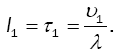 (21)
(21)
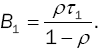
Mean Busy Cycle
The busy cycle is the time between the start of an idle period and the start of the next idle period, i.e., the difference between the starting times of two consecutive idle periods. From the theory of semi-Markov processes, see Çinlar [22], the mean length of a busy cycle is  , and therefore
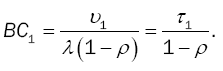 (22)
(22)
Mean Busy Period
The busy period is the time period measured between the instant a customer arrives to an empty system until the instant a customer departs leaving behind an empty system. Then, the mean length of a busy period is 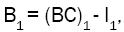 and therefore
 (23)
(23)
Probability Server is Idle
In this model, the server starts when the workload exceeds D. This means the probability of idle server is not equal to the probability of empty system as in classical queueing theory. Thus, the probability of idle server, denoted as π0, is given by:
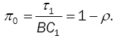 (24)
(24)
Probability Server is Busy
The probability of busy server is among the commonly used performance measures in queues to make decisions. This measure is used to measure the effectiveness of the server and is given by:
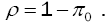 (25)
(25)
In practice, there are many applications that require a new set of performance measures other than the measures mentioned earlier. The steady-state probability of the size of the system obtained by the PGF makes it possible to express any performance measure other than the measures mentioned below.
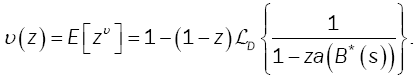
The queueing model described in this paper is considered a generalization for many other single server queueing models. The design parameters in this model, namely: the policy parameter D and the failure parameterα , give flexibility in modeling many practical situations. For example:
• Unreliable M/G/1
The PGF of this model could be easily obtained by setting D = 0 and υ(z) z . Then relation (12) becomes:
where 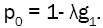 This is the pgf of the M/G/1 where the server is subject to random breakdowns.
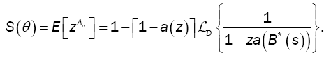
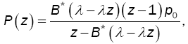
• Reliable MX/G/1 under D-policy
Setting α=0, relation (1) yields G*(s) =B*(s), and relation (12) becomes:
where 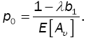 This is the pgf of the MX/G/1 where the server follows the D-policy.
• Classical M/G/1
Finally setting D = 0, υ(z)=z, and α=0, yields the well-known Pollaczeck-Khintchine formula:
where 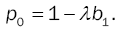
Our approach in optimization for this model is a cost driven optimization approach. Cost driven optimization uses key performance measures in a cost function then the cost function is minimized. See Tadj and Choudhury [23] for more details on queueing optimization approaches.
We, now, define the total expected cost per unit of time using some of the performance measures introduced in Section 4. The decision variable in this expression is D. The goal is to find the optimal value of this parameter that minimizes the cost function. This would optimize the performance of the system, as it would allow the server to know exactly when to end an idle period.
The total cost function of the system takes into account the total cost of holding customers in the system and the total server operation cost. It is assumed that the server needs to be setup for operation each time the server is in idle period. In addition, it is assumed that the server will perform preparatory work prior the start of each busy period. The unit cost of each cost category is given as follows:
ch: holding cost per unit time for each customer present in the system;
co: cost per unit time for keeping the server on and in operation;
cs: setup cost per busy cycle;
ca: startup cost per unit time for the preparatory work of the server before starting the service.
Then, the total expected cost function per unit time is given by
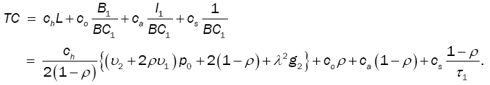
The optimal value of D is obtained using the first order optimality condition. The resulting equation is a nonlinear equation that could be solved numerically using some mathematics package.
We have considered in this paper a queueing model generalizing many of the models studied in the literature. Customerside, they are allowed to arrive in bulk. Service-side, two features. The first one is that the server is unreliable and may break down any time while providing service. The second one is that it implements the well-known D-policy.
For this model, we have obtained the PGF of the system size probabilities. We also derived many performance measures and shown how to obtain the optimal value of the threshold D.
Future research direction could include, for example, mode features from the customer side, such as balking and/or reneging, or more features from the server side, such as single or multiple vacations.
The authors are thankful to the Deanship of Scientific Research, College of Science Research Center at King Saud University for funding this research.