Keywords
|
| Software Reliability, SRGM, NHPP, imperfect debugging |
INTRODUCTION
|
| Now a day?s large and complex software systems are developed by integrating a number of small and independent modules. A system basically consists of hardware and software. Software is essentially an instrument for transforming a discrete set of input to output. Software testing begins at component level in software development phase and is usually very expensive and lengthy process as most of the commercial software products are complex systems consisting of a number of modules. So it becomes very important for the project managers to allocate specified testing resources among all the modules and develop quality software with high reliability. According to ANSI definition software reliability is defined as the probability of failure free operation for a specified period of time in a specified environment. In general it can be defined as how well the software functions to meet the requirement of customers. To predict the reliability of software many SRGM have been developed during 1970-2000. An SRGM describes failures as random process and is based on NHPP. An NHPP is a Poisson?s process with rate parameter χ(t) such that rate parameter is a function of time. It is assumed that software reliability can somehow be measured and therefore the question is that what purpose it serves. Software reliability is a useful measure in planning and controlling resources during the development process so that high quality software can be developed. It is seen that the assessed value of the reliability measure is always relative to a given user environment. In this paper two traditional SRGM models are analyzed using various parameters such as imperfect debugging and concepts of NHPP [3, 6, 7]. |
LITERATURE SURVEY
|
| In the past literature on software reliability Chin-Yu Huang in 2001 proposed an SRGM with generalized logistic TEF and elaborated a unified approach for developing software reliability growth models in the presence of imperfect debugging and error generation reliability. Dr. Ajay Gupta, Dr. Digvijay Choudhary and Dr. Sunit Saxena in 2006 discussed the software reliability estimation using delayed s-shaped model under imperfect debugging and proposed a model based testing considering cost, reliability and software quality. Xue Yang, Nan Lang & Hang Lei proposed improved NHPP model with time varying fault removing delay. Michael Grottke in 2007 analysed the software reliability model study by implementing with debugging parameters. Jang Jubhu gave an elaborate introduction to software reliability growth models using various case studies in 2008. Bruce R. Maxim in 2010 calculated the reliability of DSS model using mean time value function and some other parameters. In this paper focus was given on S shaped SRGM using a flexible modelling approach. Basically problems associated with manual operations are huge time consumption, more prone to faults and High failure rate. The proposed SRGM will replace the manual operation of analysis and complex computations with computerized one to increase the reliability. |
NOTATIONS
|
| t : time. |
| χ(t) : failure rate intensity. |
| μ(t) : mean value function. |
| N : expected total number of detected failures. |
| B : occurrence of rate of failure, proportionality constant. |
| L : reliability measure. |
| fo : expected number of initial faults. |
| fi : total number of independent faults. |
| fd : total number of dependent faults. |
| r : fault detection rate of independent faults. |
| θ : fault detection rate of dependent faults. |
| p : proportion of independent faults. |
| φ(t) : delay effect factor. |
| ψ : Inflection factor. |
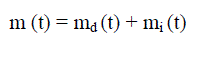
| m(t) : mean value function of expected number of faults detected. |
| md(t) : mean value function of expected number of dependent faults detected. |
| mi(t) : mean value function of expected number of independent faults detected. |
| bi : independent fault detection rate[11]. |
GOEL OKUMOTO MODEL
|
| The primary objective of Software reliability model is to predict the failure behavior of software. Goel Okumoto model provides the analytical framework for describing the software failure phenomenon during testing. |
A. Basic assumptions of Goel Okumoto Model
|
| The model proposed by Goel Okumoto is based on the following assumptions:- |
| i) The execution time between the failures is exponentially distributed. |
| ii) The cumulative number of failures by time t follows a Poisson process with mean value function μ (t). |
| iii) The number of software failures that occur in (t, t+?t) with ?t → 0 is proportional to the expected number of undetected faults, N- μ (t). The constant of proportionality is φ. |
| iv) For any finite collection of times t1<t2<t3<….<tn, the number of failures occurring in each of the disjoint intervals (0, t1),(t1, t2),(t2, t3)…(tn-1, tn) is independent. |
| v) Fault causing failure is corrected immediately otherwise reoccurrence of that failure is not counted [8]. |
| Since each fault is perfectly repaired after it has caused a failure, the number of inherent faults in the software at the beginning of testing is equal to the number of failures that will have occurred after an indefinite amount of testing. |
B. Reliability Analysis
|
| In this model, Goel and Okumoto assumed that software is subject to failures at random times caused by faults present in the system. |
| Let N (t) be the cumulative number of failures observed by time t and they proposed that N(t) can be modeled as a non homogeneous Poisson process that is a poisson process with a time dependent failure rate. |
| The proposed form of the model is as follows: |
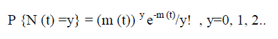 (1) (1) |
| Where m (t) =a (1-e-bt) and χ (t) = m?t = abe-bt |
| Here m (t) is the mean value function or the expected number of failures observed by time t and χ (t) is the failure intensity rate [8]. |
| A typical plot of m (t) function for the Goel Okumoto model with a= 175 and b= 0.05 is shown in figure 1. |
| In this model „a? is the expected number of failures to be observed eventually and „b? is the fault detection rate per fault. Model estimation and reliability prediction can be done using |
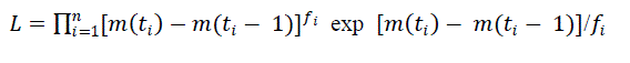 (2) (2) |
| Where fi is the failure count in each of the testing intervals and ti is the completion time of each period that the software is under observation. Plot of reliability prediction in Goel Okumoto model for a= 175 and b= 0.05 is shown below. |
DELAYED S SHAPED MODEL
|
| Reliability of software depends upon fault detection and error correction. The analysis of the problem can be made using dependent and independent faults whether the faults can be detected and corrected or not. The software reliability using this model can be analyzed by involving imperfect debugging and time delay function. |
A. Basic assumptions of Delayed S Shaped model
|
| The model proposed by Yamada is based on the following assumptions: |
| i) All detected faults are either independent that is the faults are detected and corrected immediately and there is no time delay between them or dependent that faults cannot be removed immediately. |
| ii) The software failure rate at any time is a function of fault detection rate and the number of remaining faults present at that time. |
| iii) The total number of faults is infinite. |
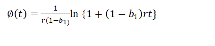
| iv) The detected dependent fault may not be removed immediately and it lags the fault detection process by ∅ ?? [2, 5]. |
B. Faults in Delayed S Shaped SRGM model
|
| Total detected faults in time (0, t) is given by: |
 (3) (3) |
i) Independent faults (mi(t))
|
| The rate of independent faults detected is proportional to the remaining faults. The differential equation is |
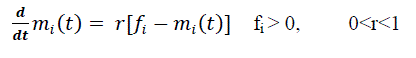 (4) (4) |
| The differential equation under imperfect debugging is |
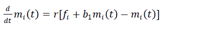 (5) (5) |
| And using time delay function Ø(t) is |
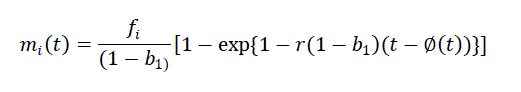 (6) (6) |
ii) Dependent faults (md(t))
|
| The rate of dependent faults detected is proportional to the remaining dependent faults in the system and the ratio of independent faults removed at time „t? to the total number of faults. |
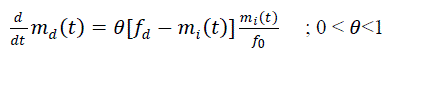 (7) (7) |
C. Reliability Analysis
|
| This model describes the S shaped curve for the cumulative number of faults detected such that the failure rate initially increases and later decreases. |
 (8) (8) |
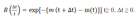
| The software reliability is defined as the probability that a software failure does not occur in the time interval (t, t + Δt): |
 (9) (9) |
| The number of failures m (t) and software reliability R(t) have been evaluated considering the input as f0= 400, r= 0.255, θ= 0.0833, ψ= 2.84, p=0.55, b=0.1, fi=0, 1, 2…. |
| Fig.3 represents the variation of number of faults detected with respect to time. Initially the faults detected during testing are very high but later on becomes constant. The number of faults debugged under imperfect debugging is higher than that in perfect debugging. |
| Fig.4 represents the variation of software reliability with respect to testing time. Software reliability increases rapidly with testing time during initial phase. If we incorporate the factors like faults dependency, debugging time lag and imperfect debugging into model, prediction of software reliability is more realistic and generalized. |
CONCLUSION
|
| In this paper a review of software reliability growth models is presented. Two classes of analytical models along with their underlying assumptions were described. It should be noted that the above analytical models are primarily useful in estimating and monitoring software reliability. A generalized framework for software reliability growth modeling is analyzed with respect to testing effort and faults of different severity. Software reliability growth model can provide a good prediction of number of faults at a particular time and can compute the remaining numbers of failures also. When the software is at high risk, the testing effort would be too high and the rate of detection of errors would be high and value of „b? would approach to 1 and hence reliable software can be produced. The present study is based on assumption of independence of failures of modules and in future the dependence of failures from different modules can also be considered and reliability can be studied. |
|
Figures at a glance
|
 |
 |
 |
 |
| Figure 1 |
Figure 2 |
Figure 3 |
Figure 4 |
|
| |
References
|
- C.Y Hung, M. R Lyu, and S. Y Kuo, “A unified scheme of some non-homogeneous poison process models for Software reliability estimation”, IEEE transaction on Software Engineering, Vol 29,Issue.3, pp. 261-269,2003.
- P.K Kanpu , H. Pham, S. Anand and K .Yadav, “An Unified approach for developing software reliability growth models in the presence of imperfect debugging and error generation reliability”, IEEE transaction ,Vol.6, Issue 1, pp. 331-340,2003.
- M.R Lyu, “Handbook of software reliability engineering”, McGraw Hill, pp.428-443, 1993.
- L Goel and K. Okumoto “Time dependent error detection rate model for software reliability and other performance measures” IEEE transaction on reliability, Vol 28, Issue.3, pp 206-211, 1979.
- H. Hetaera and S. Yamada, “Optimal allocation and control problems for software testing resources”, IEEE transaction on reliability, Vol.39, Issue. 2, pp 171-176, 1990.
- P. Kubat and H.S Koch, “Managing test procedure to achieve to achieve reliable software”, IEEE transaction on reliability, Vol 32, Issue 3, pp-299- 303, 1983.
- B. Littlewoods, Software reliability growth model for modular programming structure. IEEE transaction on reliability. Vol. 28, Issue 3, PP-35-41, 1989.
- P. Nagar and B. Thankachan, “Application of Goel-Okumoto Model in Software Reliability Measurement”, International Journal of Computer Applications, Vol.30, Issue 2, pp 0975 – 8887, 2012.
- B.W Boehm, J.R Brown, and M. Lipow, “Quantitative evaluation of software quality”, In proceeding 2nd International conference software engineering, Sanfrancisco, CA, Vol. 26, Issue. 3 PP-592-605, 1986.
- C.V Ramamoorthy and F.B Batsani, “Software reliability: status and prospectives”, IEEE transaction on software engineering, Vol. 8,Issue 2, pp-359-371, 1982.
- C.Y Huang and M. R. Lyu, “Optimal Testing Resource Allocation, and Sensitivity Analysis in Software Development”, IEEE transactions on reliability, vol. 54, Issue 4, December 2005
|