Benyammi Youcef1, Moussi Oumelkeir2*
1Department of Economics, Business and Management, University of Algiers 3, Alger, Algeria
2Department of Economics, Ecole Nationale Supérieure de la Statistique et d’Economie Appliquée(ENSSEA),France
Received date: 30/12/2015; Accepted date: 28/01/2016; Published date: 03/02/2016
Visit for more related articles at Research & Reviews: Journal of Statistics and Mathematical Sciences
Usually we use the Dickey-Fuller test for testing stationarity in a time series under the hypotheses H0: I (1) (presence of unit root) versus H1: I (0) (absence of unit root), and it is used in the case of a short memory. In this article, we propose an extension of the fractional Dickey-Fuller test proposed by Bensalma used in the long memory case and when the errors of test regression are autocorrelated. The proposed test is considered as a generalization of ADF test and they have the same steps. The asymptotic properties of this test are derived and it is studied by Monte Carlo simulation experiment. The paper ends with an application to illustrate the usefulness and the simplicity of the proposed technique.
ARFIMA, Long memory, Test of fractional parameters, FDF test
Considering the importance of the identification of the fractional integration parameter, many researchers are interested by the statistical tests based on this parameter. These tests are revealed very useful to capture the persistence properties of many long memory processes. The stationnarity tests are often the subject of several papers. There is a growing number of works which develop new approaches of these tests. These works were made in a way to verify the belonging of the parameter d, such that if d < 1/ 2 the process is stationary (asymptotically stationary) and if d ≥ 1/ 2 the process is not stationary.
At the beginning, the Hurst statistics is used as a heuristic test to test the presence of a long memory behavior, then, with the development of the stochastic approach, other tests have been exposed in order to improve the performance of these tests. Among these tests we find the GPH test (Geweke and Porter-Hudak test) which is developed to test in frequency domain the presence of long memory. Robinson and Tanaka have proposed Lagrange Multiplier test (LM test) in the frequency and the time domain respectively. Another type of test is proposed by Dolado [1], Gonzalo and Mayoral and modified by Lobato and Velasco [2], since it is a Wald type test that working under the alternative assumption. This test is called fractional Dickey-Fuller test (FDF test), originally developed for the case FI(d0) versus FI(d1) with d1 < d0. Lately, Bensalma [3] have proposed a statistical test that has acceptable power properties and based on the principle of Dickey-Fuller which test the presence of unit root. It turns out to be a generalization of the well-known Dickey-Fuller (D-F) test, and can be seen as better than FDF in terms of simplicity, efficiency and implementation..
All the steps and the properties of the Bensalma-test are similar to the Dickey-Fuller test, moreover, the hypotheses which he used are the same as DF test. Thus, he has proved that we can use the critical values found by Dickey fuller to execute his test. For this reason, we proceeded to the development of fractional Dickey Fuller test presented by A. Bensalma [3] in the augmented case. This development was made by Monte Carlo simulation methods to study the performance (power), and check the empirical distribution.
This article is organized as follows. In the next section, we introduce the new fractional Dickey-Fuller test presented by Bensalma [3]. In Section 3, we discuss about the new fractional augmented Dickey-Fuller test in several subsections. In the first, we introduce the regression which is uses in the test. Secondly, we study the asymptotic distribution of test statistic and calculate the critical value. The last subsections, contains the Monte Carlo simulation experiment, where size and power of the tests are studied. Section 4 discusses of an empirical application of the previous test. Finally, Section 5 summarizes the conclusions.
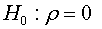
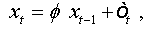
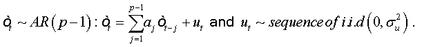
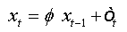
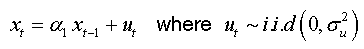
Bensalma [4] proposed a new test based on the fractional parameter inspired, essentially, by the well-known Dickey-Fuller test [5], but in a more general case (fractional case). This test was developed under the assumptions:
The regression test is given by:
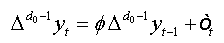 (1)
(1)
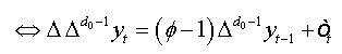
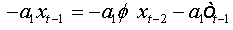
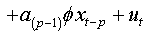
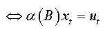
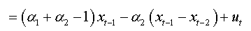
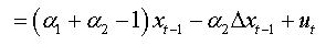
The equation (01) can be written as:
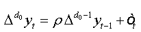 (2)
(2)
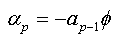
where ρ =φ −1
The assumptions test can be built in basing of the coefficient ρ from the regression presented in (02) as:

The asymptotic distribution of the OLS estimator of ρ and its t-ration under the null hypothesis it given by the following theorem:
Theorem:
If  is a data generating process defined by:
  , and let be the regression presented in (02)
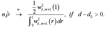
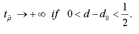
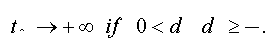
When n → +∞ , we have:
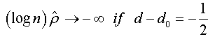
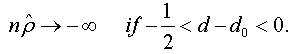
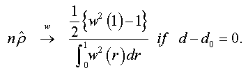
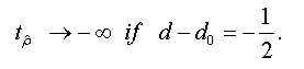
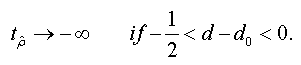
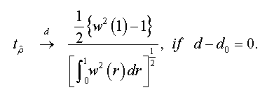
And when n → +∞ , the t-stat verifies that:
 <
< 
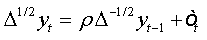
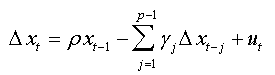
To test the asymptotic stationarity in a fractional time series we use the following test problem: H0: d≥ ½ against H1 : d > 1/2 The auxiliary regression test is given by:
Under the assumptions that d=1 and 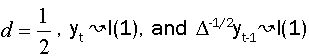 respectively, and the both cases are similar to conventional test [5]. Thus, the corresponding asymptotic distributions, under d=d0, are invariant and similar to those given by Dickey and Fuller [5]. Therefore, the critical values obtained from asymptotic distribution are identical which found by Fuller [6] and presented after by Mackinnon.
Furthermore, all the steps of this test and the given theoretical results have been verified by Monte Carlo simulations in his article, which leaves suggest that this test is a powerful tool to test stationarity in the fractional case.
The asymptotic distributions of NFDF test statistic test were studied under the assumption that the error term ( òt ) in regression (02) is white noise. But, this assumption is not always verified.
In this section, we based on the results obtained by Bensalma [4], to extend his principle results in case where the errors are serially correlated.
Transformation model
Let ( yt, t ∈Z) be fractional process and: 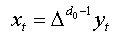 (4)
(4)
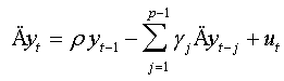
The auxiliary regression presented in (01) can be written in the following form: 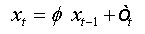 (5)
(5)
where 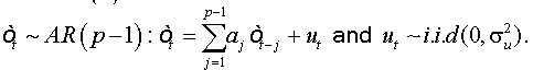
Although, the errors are auto-correlated, and in order to reduce to a regression with non-auto-correlated errors, we must perform the following lemma:
Lemma
Any AR (1) - process with auto-correlated errors of order (p), can be reduced to an AR (p) with non-auto-correlated errors.
Consequences of the lemma
Any AR (k) - process with auto-correlated errors of order (p-k) can be reduced to an AR (p) with non-auto-correlated errors.
Proof: see Appendix
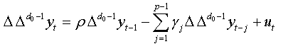
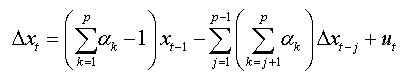
From this lemma and its consequences we found that equation (05) can be written in the form below
 (6)
(6)
Where 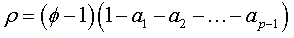
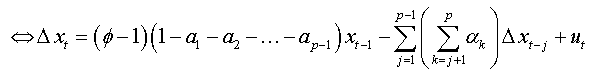
We replace xt by the expression (04):
This equation is equivalent to:
Remarks:
This equation represents the augmented regression of NFDF test presented by Bensalma [3].
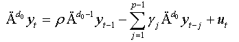
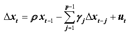
(i) If the coefficients γj are not significant, we will have the simple model of NFDF test:
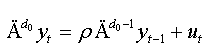
(ii) If d0=1, thus:
This model represents the regression of classical Augmented Dickey-Fuller test. Thus, this test can be considered as generalization of Augmented Dickey-Fuller test [7] and is based on significance of coefficient ρ in regression (07).
Monte-carlo experiments:
Hereinafter, we study the analogy of the test in the augmented case by Monte Carlo simulation experiments using some approaches used in the NFDF test presented above.
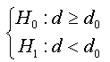
Reconstruction of the assumptions test:
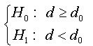
Consider the following testing problem: H0: d ≥ d0 vs H1: d < d0, These assumptions can be constructed as function of coefficient ρ of augmented regression presented in (07) and this reformulation is presented in the following proposition:
Proposal 01:
Under the null hypothesis (where d ≥ d0), the OLS estimator of coefficientρ, ρˆ , in regression (07) is zero.
Under the alternative hypothesis (where d < d0) the OLS estimator of coefficient ρ, ρˆ ,in regression (07) is strictly less than zero, and it converges to the infinity when d0 is great.
We can simplify this proposal as follows:
Under the stated proposition, tests 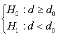 amounts to testing
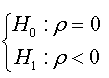
from the regression (07).
Proof
The Proof of this proposal will be made using simulations:
The experiment covers ARFIMA(1,d,0) series of length T=500 for several values of d (d=1,0.25,0.5,0.75,1,1.25,1.2,2). The Monte Carlo study involves 1000 replicates (series), where in each series we calculate the estimator of ρ.
Figure 1 below shows the smoothed curves of estimated ρ.

Figure 1: The convergence of the coefficient ρ according to the values of d (d=0,0.25,...2) and d0 of ARFIMA (1,d,0) processes.
The equivalence of the first two hypotheses, and second, is very clear in Figure 1, such as when we fixed d at d=1,0.25,0.5,0.75,1,1.25,1.2,2, the value of ρ is 0 for any values of d0 ≤ d. As soon as d0 takes values higher than d, the values of ρˆ start to decrease and they take negative values. For example, consider the Figure 1d, we note that the coefficient ρˆ is equal to zero when d0^0.75(until the discontinuous red line where d = d0). From this point, the values of start to decrease with negative values, what confirms that the hypothesis ρˆ = 0 is equivalent to d ≥ d0, as well as the alternative assumption ρˆ < 0 is equivalent to the d > d0.
Under the null hypothesis, Said and Dickey [8] showed that the asymptotic distribution of test statistic in the augmented case is identical to that derived in simple case (absence of the errors autocorrelation). Moreover, Bensalma showed that the distribution of DF test statistic is similar to NFDF test when d = d0. The asymptotic distribution behavior of test statistic of NFDF test is given in the following proposition.
Proposal 02:
Under the assumption that: d = d0, the asymptotic distribution of NFADF test statistic is invariant and identical to the distribution of ADF test statistic.
i.e., if the value of d0 is equal to the true value of integration (whatever this value), the distribution remains same and identical one to the ADF test.
Proof:
The Proof is made in a way to compare the empirical distributions of NFADF and ADF tests. This comparison is made specifically on the quantiles (critical values) of the various distributions.
The simulation experiments, presented here, are as follows:
a. First, our objective is to generate several processes (corresponding to ARFIMA (0,d, 0) and ARFIMA(p,d,0)).
b. These models are based on fractional noise series which generated using the algorithm of Diebold and Rudebusch.
c. The regression test (07) was estimated by putting d = d0 = 1/2, to assure the condition of similarity between the both distributions DF and NFDF.
d. The estimated quantiles (critical values) of NFDF test and NFADF test (with lags varying from one to five); Significance level ranging from 0.01 to 0.99 and for different sample sizes T= 25, 50, 100, 150, 200, 500, 1000, 3000) are obtained from an arithmetic average of 50 simulation experiments, each one containing 10,000 replications.
The distribution of NFADF test statistic is different from the normal distribution of the same expectation and same variance (Figure 2a), and this is confirmed by the Q-Q-plot presented in the Figure 2b which lets suggest that the distribution of the test statistic does not normally distributed.

Figure 2: comparing the empirical distribution of ADF test with normal distribution and the empirical distribution of ADF test.
The Figures 2c and 2d represent the plots of the empirical distributions of the ADF and NFADF test statistic, and the distribution of nρˆ of test ADF and NFADF respectively. Note that there is a perfect superposition of the distributions, which confirms the statement of our proposition.
The table of critical values is given in the appendix.
From the table of estimated critical values (09):
• We see that these values are quasi-similar with the usual tabulated critical values obtained by Dickey-Fuller [5], Dickey and Said [8] and by J MacKinnon.
• On the other hand the critical values for the same sample size, for different numbers of lags, and for the same threshold are very close from one to another.
Hence, the choice of a single value for all lags is suitable; therefore we chose the average of critical values as the representative value (Table 1).
| T | Probability that  be less than C(α) be less than C(α) |
|||||||
|---|---|---|---|---|---|---|---|---|
| 0.01 | 0.025 | 0.05 | 0.1 | 0.9 | 0.95 | 0.975 | 0.99 | |
| 25 | -2.665 | -2.287 | -1.956 | -1.614 | 0.916 | 1.321 | 1.689 | 2.093 |
| 50 | -2.625 | -2.263 | -1.948 | -1.626 | 0.904 | 1.309 | 1.635 | 2.064 |
| 100 | -2.599 | -2.253 | -1.946 | -1.618 | 0.900 | 1.297 | 1.636 | 2.015 |
| 150 | -2.585 | -2.251 | -1.946 | -1.615 | 0.899 | 1.291 | 1.635 | 2.035 |
| 250 | -2.590 | -2.247 | -1.944 | -1.615 | 0.891 | 1.284 | 1.613 | 2.031 |
| 500 | -2.581 | -2.223 | -1.941 | -1.611 | 0.885 | 1.284 | 1.614 | 2.003 |
| 1000 | -2.564 | -2.229 | -1.944 | -1.613 | 0.888 | 1.296 | 1.633 | 2.051 |
| 3000 | -2.563 | -2.16 | -1.940 | -1.613 | 0.883 | 1.289 | 1.612 | 2.047 |
Source: made by ourselves from simulations
Table 1: Estimated critical values of the new fractional Dickey-Fuller test statistic.
Power and size of NFADF test:
In the next, we will study the reliability of the test in the augmented case by analyzing the size and power of several models ARFIMA (p, d, 0).
Proposition 04:
Let yt,t∈ Z be random process, andα,β are the first and second type-errors respectively of new fractional augmented Dickey Fuller test whose assumptions are given by:
there exists an unbiased test determined by the critical region Wα,
with 
and 
where t is the test statistic corresponding to ρˆ ,d defined as:  , and cn(α )is the critical value at level α
Proof:
To prove the proposition, we will proceed to Monte Carlo simulations of several ARFIMA(p,d,0) models, where we took different values of d(d = 0, 0.5 ,1)) to check all possible cases (Memory long and short memory, stationary and non-stationary).
We took into account several lags of the Autoregressive part of these processes (p=1,2,3,4), and the values of coefficients were selected in a random way under the assumption of stationarity of the autoregressive part.
We will study the size and the power of NFADF test at the thresholds 1%, 5% and 10% of the different simulated models with various sample sizes(T= 25,50,100,300 et 1000) and for several values of d0 (d0 ∈]-1.5,1],).
For each experiment we used 10000 replications and the results are presented in the following tables.
Preliminary result:
We conducted several simulation experiments and we noticed that we get the same results when changing the number of lags used to run the test and when changing the coefficient of the autoregressive part. Therefore, in our study presented below, we chose an augmented model with only one lag.
The following Tables 2-7 present the calculated sizes and powers of the NFDF test using simulation methods of Monte Carlo with assumptions discussed above.
| T | α\d0 | 0 | -0.1 | -0.2 | -0.3 | -0.4 |
|---|---|---|---|---|---|---|
| 25 | 1% | 98.1 % | 99.3 % | 99.8 % | 99.7 % | 99.9 % |
| 5% | 94.4 % | 96.2 % | 98.3 % | 98.8 % | 98.6 % | |
| 10% | 89.5 % | 93.3 % | 95.2 % | 97.2 % | 96.3 % | |
| 50 | 1% | 99.3 % | 99.5 % | 99.7 % | 99.9 % | 100 % |
| 5% | 95.4 % | 97 % | 98.4 % | 99.3 % | 99.4 % | |
| 10% | 89.4 % | 93.6 % | 96.4 % | 98.4 % | 98 % | |
| 100 | 1% | 99 % | 99.8 % | 99.9 % | 100 % | 100 % |
| 5% | 94.5 % | 97.6 % | 99.3 % | 99.6 % | 100 % | |
| 10% | 89.6 % | 95.3 % | 97.4 % | 98.6 % | 99.6 % | |
| 500 | 1% | 98.9 % | 99.9 % | 100 % | 100 % | 100 % |
| 5% | 95.1 % | 98.9 % | 99.9 % | 100 % | 100 % | |
| 10% | 91 % | 97.2 % | 99.2 % | 100 % | 100 % | |
| 1000 | 1% | 98.9 % | 99.9 % | 99.9 % | 100 % | 100 % |
| 5% | 94.7 % | 99.3 % | 99.7 % | 100 % | 100 % | |
| 10% | 89.8 % | 98.2 % | 99.5 % | 99.9 % | 100 % |
Source: made by ourselves from simulations
Table 2: Calculated probability of accepting H0: d = 0 ≥ d0 (size), based on the asymptotic quantiles 1%, 5% and 10% of the Dickey-Fuller distribution calculated by JG MacKinnon.
| T | α\d0 | 0.5 | 0.4 | 0.3 | 0.2 | 0.1 |
|---|---|---|---|---|---|---|
| 25 | 1% | 99.2 % | 99.6 % | 99.7 % | 99.6 % | 100 % |
| 5% | 95.1 % | 96.9 % | 97.2 % | 97.8 % | 98.9 % | |
| 10% | 89.9 % | 93.5 % | 94.5 % | 95.3 % | 97.2 % | |
| 50 | 1% | 99.1 % | 99.3 % | 99.8 % | 100 % | 100 % |
| 5% | 95.5 % | 97.1 % | 99 % | 99.6 % | 99.5 % | |
| 10% | 90.6 % | 93.3 % | 96.7 % | 97.3 % | 98.5 % | |
| 100 | 1% | 99.1 % | 99.6 % | 99.8 % | 100 % | 100 % |
| 5% | 95.3 % | 98.1 % | 99.3 % | 99.8 % | 100 % | |
| 10% | 90.1 % | 95.4 % | 97.3 % | 99.3 % | 99.7 % | |
| 500 | 1% | 99.2 % | 100 % | 100 % | 100 % | 100 % |
| 5% | 95.3 % | 98.8 % | 99.6 % | 99.9 % | 100 % | |
| 10% | 90.6 % | 97.3 % | 99.3 % | 99.9 % | 99.9 % | |
| 1000 | 1% | 99.2 % | 99.9 % | 100 % | 100 % | 100 % |
| 5% | 94.9 % | 99.6 % | 100 % | 100 % | 100 % | |
| 10% | 90.9 % | 98.4 % | 99.9 % | 100 % | 100 % |
Source: made by ourselves from simulations
Table 3: Calculated probability of accepting H0: d = 0.5 ≥ d0 (size) based on the asymptotic quantiles 1%, 5% and 10% of the Dickey-Fuller distribution calculated by JG MacKinnon.
| T | α\d0 | 1 | 0.9 | 0.8 | 0.7 | 0.6 |
|---|---|---|---|---|---|---|
| 25 | 1% | 99.1 % | 99.2 % | 99.8 % | 99.8 % | 99.9 % |
| 5% | 95.4 % | 96.3 % | 97.6 % | 97.8 % | 98.1 % | |
| 10% | 90.9 % | 92.6 % | 94.3 % | 95.5 % | 96.1 % | |
| 50 | 1% | 99.1 % | 99.4 % | 99.8 % | 99.8 % | 100 % |
| 5% | 95.1 % | 97.2 % | 98.3 % | 99 % | 99.3 % | |
| 10% | 89.5 % | 93.9 % | 96 % | 97.5 % | 98.1 % | |
| 100 | 1% | 98.5 % | 99.7 % | 99.8 % | 99.9 % | 100 % |
| 5% | 94.4 % | 97.9 % | 99 % | 98.9 % | 99.9 % | |
| 10% | 89.9 % | 95.7 % | 97.1 % | 98.2 % | 99.3 % | |
| 500 | 1% | 98.9 % | 99.9 % | 100 % | 100 % | 100 % |
| 5% | 95.2 % | 98.9 % | 99.8 % | 100 % | 100 % | |
| 10% | 90.5 % | 97 % | 99.3 % | 100 % | 100 % | |
| 1000 | 1% | 99.2 % | 99.8 % | 100 % | 100 % | 100 % |
| 5% | 94.8 % | 99.3 % | 100 % | 100 % | 100 % | |
| 10% | 89.8 % | 98.1 % | 997 % | 100 % | 100 % |
Source: made by ourselves from simulations
Table 4: Calculated probability of accepting H0: d = 1 ≥ d0 (size), based on the asymptotic quantiles 1%, 5% and 10% of the Dickey-Fuller distribution calculated by JG MacKinnon.
| T | α\d0 | 0.1 | 0.2 | 0.3 | 0.4 | 1 |
|---|---|---|---|---|---|---|
| 25 | 1% | 02.1 % | 03.9 % | 04.0 % | 08.6 % | 83.2 % |
| 5% | 08.0 % | 14.5 % | 16.3 % | 26.6 % | 98.5 % | |
| 10% | 14.6 % | 23.5 % | 28.1 % | 40.7 % | 99.6 % | |
| 50 | 1% | 02.6 % | 04.3 % | 11.0 % | 20.6 % | 99.8 % |
| 5% | 11.2 % | 15.7 % | 28.2 % | 49.4 % | 100 % | |
| 10% | 19.1 % | 28.1 % | 43.5 % | 66.4 % | 100 % | |
| 100 | 1% | 02.5 % | 09.5 % | 24.0 % | 44.7 % | 100 % |
| 5% | 10.4 % | 25.7 % | 47.1 % | 71.9 % | 100 % | |
| 10% | 19.6 % | 37.7 % | 62.6 % | 82.9 % | 100 % | |
| 500 | 1% | 6.9 % | 29.3 % | 66 % | 95.3 % | 100 % |
| 5% | 19.6 % | 50.3 % | 84.4 % | 99.2 % | 100 % | |
| 10% | 31.2 % | 64.4 % | 91.5 % | 99.8 % | 100 % | |
| 1000 | 1% | 8.8 % | 38 % | 83 % | 99.3 % | 100 % |
| 5% | 22.6 % | 60.8 % | 93.8 % | 99.9 % | 100 % | |
| 10% | 34 % | 72.5 % | 97.1 % | 100 % | 100 % |
Source: made by ourselves from simulations
Table 5: Calculated probability of accepting H1: d = 1 < d0 (power), based on the asymptotic quantiles 1%, 5% and 10% of the Dickey -Fuller distribution calculated by JG MacKinnon.
| T | α\d0 | 0.6 | 0.7 | 0.8 | 0.9 | 1.5 |
|---|---|---|---|---|---|---|
| 25 | 1% | 01.9 % | 02.9 % | 05.6 % | 08.1 % | 83.9 % |
| 5% | 08.6 % | 10.3 % | 19.6 % | 28.5 % | 92.1 % | |
| 10% | 14.8 % | 19.7 % | 30.3 % | 44.3 % | 96.2 % | |
| 50 | 1% | 03.7 % | 06.5 % | 10.9 % | 22.6 % | 100 % |
| 5% | 10.8 % | 17.4 % | 31.6 % | 48.6 % | 100 % | |
| 10% | 17.8 % | 28.8 % | 46.8 % | 63.8 % | 100 % | |
| 100 | 1% | 02.6 % | 08.5 % | 22.5 % | 44.9 % | 100 % |
| 5% | 11.8 % | 22.1 % | 47.8 % | 72.8 % | 100 % | |
| 10% | 20.1 % | 35.2 % | 60.6 % | 84.0 % | 100 % | |
| 500 | 1% | 07.5 % | 67.4 % | 30.1 % | 95.7 % | 100 % |
| 5% | 19.5 % | 85.1 % | 50.9 % | 99.3 % | 100 % | |
| 10% | 29.9 % | 90.8 % | 63.5 % | 99.8 % | 100 % | |
| 1000 | 1% | 09.1 % | 35.6 % | 84.2 % | 99.0 % | 100 % |
| 5% | 23.8 % | 58.1 % | 94.4 % | 100 % | 100 % | |
| 10% | 35.4 % | 70.3 % | 97.4 % | 100 % | 100 % |
Source: made by ourselves from simulations
Table 6: Calculated probability of accepting H1: d = 0.5 < d0 (power), based on the asymptotic quantiles 1%, 5% and 10% of the Dickey-Fuller distribution calculated by JG MacKinnon.
| T | α\d0 | 1.1 | 1.2 | 1.3 | 1.4 | 2 |
|---|---|---|---|---|---|---|
| 25 | 1% | 1.8 % | 1.8 % | 5.8 % | 7.1 % | 84.5 % |
| 5% | 7.4 % | 10.9 % | 20.5 % | 28.4 % | 97.7 % | |
| 10% | 15.7 % | 21.6 % | 33.9 % | 43.9 % | 99.4 % | |
| 50 | 1% | 1.4 % | 6.2 % | 10.1 % | 20.6 % | 100 % |
| 5% | 8.7 % | 17.7 % | 29.6 % | 48.6 % | 100 % | |
| 10% | 14.8 % | 27.7 % | 42.9 % | 64.8 % | 100 % | |
| 100 | 1% | 2.7 % | 8.4 % | 22.1 % | 43.6 % | 100 % |
| 5% | 11.8 % | 24.5 % | 47.2 % | 71.2 % | 100 % | |
| 10% | 20.1 % | 36.2 % | 63.2 % | 82.9 % | 100 % | |
| 500 | 1% | 7.3 % | 27.2 % | 62.6 % | 95.5 % | 100 % |
| 5% | 20.8 % | 49.2 % | 81.2 % | 99.8 % | 100 % | |
| 10% | 30.2 % | 62.4 % | 88.6 % | 100 % | 100 % | |
| 1000 | 1% | 9.8 % | 37.5 % | 81.9 % | 99.2 % | 100 % |
| 5% | 24.9 % | 61.5 % | 92.1 % | 100 % | 100 % | |
| 10% | 34.6 % | 71.6 % | 96.2 % | 100 % | 100 % |
Source: made by ourselves from simulations
Table 7: Calculated probability of accepting H1: d = 1 < d0 (power), based on the asymptotic quantiles 1%, 5% and 10% of the Dickey -Fuller distribution calculated by JG MacKinnon.
From the first three tables, we note that:
Under H0, when d0 = d, the probability of accepting the null hypothesis is close to the value (1- α), ∀α= 1%, 5% et 10% (first column of the first Table 3) with a gap which does not exceed 1%, what confirms the similarity of this distribution (NFADF test) with ADF test.
• For other values of d0, the results obtained show that whenever they move away from d (real value), the probability of accepting H0 increases until it reaches 100% (for large sample sizes). This will ensure accurate decision in the choice of null hypothesis in the different practical experiences.
In the tables where we calculated the powers (Tables 4,5 and 6):
• The link between α (type I error) and the power is well defined, so that when we take a higher value of α, the power increases and vice versa.
• Note that the power is low, when we rises α or when we increase the sample length. But in all the cases it remains higher than α. Take α = 1% as an example, all the calculated powers, whatever the sample and whatever the values of d et d0, are higher than 1% (same remarks for α = 5% and α = 10%). This means that this statistical test is an unbiased test.
• We also note that the powers reach 100% when the difference between d et d0 is great, and especially when the sample size is large.
From this remarks and results, we can say that this proprieties are similar than which found by Said and Dickey (1984).
Empirical applications
In what follows, we will apply the new fractional Dickey-Fuller test on data of the Nile river which evidence of long memory has been proved before in the other studies, and is well characterized by a stationary fractional white noise 0 < d < 1/2.
We consider the yearly minimal water levels of the Nile River for the years 622-1281 A.D, measured at the Roda Gauge near Cairo and contain 663 observations. These data were taken from the book of Tousson [9]; the measuring unit presented by Beran [10] is the centimeter.
The presence of long memory in the Nile River minima can be seen in Figure 3a. It indicates that the plot of the autocorrelations suggests a slow decay of the correlations (Figure 3b). Similarly, the theoretical spectral density of this series exhibits a pole at zero frequency (Figure 3c).

Figure 3: Nile River minima: Yearly minimum water levels (Fig 03.a); sample autocorrelations (Fig 03.b); smoothed periodogram (Fig 03.c).
Further evidence for this type long-range dependence behaviour is given by the modified R/S statistic and Whittle estimator of d, where we are found that the estimated of Hurst statistic for this series is:  =0.876, and as H= d+1/2, the value of the fractional is
  =0.376. Moreover, the Whittle estimator parameter of an ARFIMA (0,d,0) is:
  =0.4202.
To test stationarity in long memory case it suffices to put d0 = 1/2, in the test hypotheses of H0: d ≥ 1/2 against H1: d > 1/2. It will be: of H0: d ≥ 1/2 against H1: d < 1/2.
We can try to identify the lags in test regression by identifying the maximum order (p.max) from the periodogram of the partial autocorrelation function, and then we use the usual Akaike information criterion (AIC) and the Schwarz information criterion (SIC).
The following table presents the results of applying the NFADF test to different estimated models based on the number of lags.
From this table, one notes that the adequate regression of the test is that which has no lag and arises as follows:
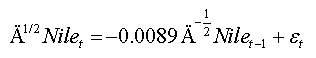
Note that the value of this statistic is greater than the tabulated critical value (Table 8) at level 5% (-1.941), in this case we must reject the null hypothesis of non-stationarity of the series, a result that agrees with those obtained by estimation of fractional parameter presented above and with those obtained by Beran (1994).
 |
 -stat -stat |
AIC | SIC | |
|---|---|---|---|---|
| Lags | ||||
| P=0 | -0.012268 | -2.004 | 11.34920 | 11.36278 |
| P=1 | -0.011523 | -1.878* | 11.36597 | 11.38637 |
| P=2 | -0.010417 | -1.698* | 11.36095 | 11.38818 |
| P=3 | -0.010014 | -1.628* | 11.36362 | 11.39770 |
| P=4 | -0.009912 | -1.605* | 11.36807 | 11.40902 |
| P=5 | -0.009674 | -1.567* | 11.36319 | 11.41102 |
| P = 6 | -0.008924 | -1.456* | 11.36530 | 11.40003 |
(*) denote rejection of the null hypothesis at the 5% level, using the ADF critical values.
Table 8: Estimated of NFADF test regressions for different lags of the Nile River series.
From this application we can deduce that this is test simple to compute and has the same procedure testing as ADF test. An advantage of using this test is that is standard where we can use it in the both cases short and long memory.
In this article we proposed New Fractional Augmented Dickey-Fuller test of H0 : d ≥ ½ against H1 : d < 1/2, based essentially on New Fractional Dickey-Fuller test presented by Bensalma (2013) Which also inspired from Dickey-Fuller test (1979). This test is considered as a generalization of ADF test (1984), such that if d0 = 1 this fractional test regression is reduced to the simple ADF test regression presented by Said and Dickey (1984). Moreover, it was shown that if the true value is equal to d0 (d = d0), the distribution of the test statistic is identical to ADF test.
The NFADF has great power in large samples and by using the simulation experiments we get a test which is unbiased for any values of significance level. In general, the proprieties of NFADF test is close to the proprieties of the ADF test (1984).
Finally, an empirical illustration is provided for show how to use this test and for put the interests of using the fractional Dickey-Fuller test seen its simplicity and flexibility of use.
Proof of lemma:
Let ( xt,t∈Z be an AR(1) process which is written as:
where
The errors are auto-correlated by their definition. To reduce to a regression with non-correlated errors we must perform the following transformation:
Summing equations, we obtain:


And as: 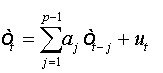

 (1a)
(1a)
 (2a)
(2a)
where  is a characteristic polynomial with all its roots are outside the unit circle.
We note that this regression (2.a) is that of an autoregressive model of order (p) with no auto-correlated errors.
Proof of Consequences of the lemma
To simplify the demonstration let us take autoregressive models with coefficients easier to handle than those of the previous expression (1.a) which depend on the φ and a:
For an AR(1):
We can write: 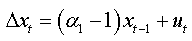
For an AR(2):

We can write: 
For an AR(3):

We can write:


For an AR(p):

We can write in same way:
 (1b)
(1b)
We will replace the coefficients αk of this expression with the values found in the expression (1.a), we obtain:
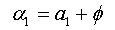
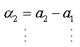
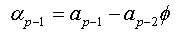
The expression (1.b) becomes:

We factorize by Φ the first bracket of the right-hand side, and we obtain:


So:
Critical values:
| T | Lag (p) | La probabilité que  est inférieure à C(α) est inférieure à C(α) |
|||||||
|---|---|---|---|---|---|---|---|---|---|
| 0.01 | 0.025 | 0.05 | 0.1 | 0.9 | 0.95 | 0.975 | 0.99 | ||
| 25 | 0 | -2,698 | -2,279 | -1,957 | -1,61 | 0.913 | 1.324 | 1.699 | 2.099 |
| 1 | -2,670 | -2,291 | -1,964 | -1,615 | 0.926 | 1.332 | 1.692 | 2.094 | |
| 2 | -2,645 | -2,287 | -1,955 | -1,611 | 0.910 | 1.315 | 1.672 | 2.084 | |
| 3 | -2,642 | -2,287 | -1,957 | -1,62 | 0.921 | 1.329 | 1.686 | 2.101 | |
| 4 | -2,651 | -2,289 | -1,951 | -1,617 | 0.912 | 1.306 | 1.694 | 2.091 | |
| 5 | -2,688 | -2,292 | -1,952 | -1,611 | 0.916 | 1.324 | 1.694 | 2.093 | |
| 50 | 0 | -2.624 | -2.247 | -1.950 | -1.631 | 0.899 | 1.310 | 1.641 | 2,059 |
| 1 | -2.623 | -2.270 | -1.949 | -1.645 | 0.885 | 1.269 | 1.630 | 2,061 | |
| 2 | -2.624 | -2.264 | -1.952 | -1.624 | 0.911 | 1.344 | 1.632 | 2,086 | |
| 3 | -2.629 | -2.267 | -1.948 | -1.618 | 0.905 | 1.321 | 1.636 | 2,066 | |
| 4 | -2.631 | -2.270 | -1.945 | -1.617 | 0.916 | 1.305 | 1.642 | 2,058 | |
| 5 | -2.620 | -2.261 | -1.948 | -1.622 | 0.909 | 1.309 | 1.629 | 2,054 | |
| 100 | 0 | -2.574 | -2.278 | -1.940 | -1.613 | 0.897 | 1.304 | 1.639 | 2.022 |
| 1 | -2.625 | -2.258 | -1.940 | -1.632 | 0.877 | 1.287 | 1.619 | 1.936 | |
| 2 | -2.602 | -2.257 | -1.948 | -1.615 | 0.912 | 1.298 | 1.646 | 2.034 | |
| 3 | -2.595 | -2.237 | -1.945 | -1.621 | 0.907 | 1.302 | 1.637 | 2.042 | |
| 4 | -2.598 | -2.241 | -1.951 | -1.617 | 0.899 | 1.289 | 1.640 | 2.045 | |
| 5 | -2.600 | -2.247 | -1.952 | -1.615 | 0.901 | 1.307 | 1.635 | 2.038 | |
| 150 | 0 | -2.581 | -2.263 | -1.943 | -1.618 | 0.903 | 1.298 | 1.639 | 2.041 |
| 1 | -2.566 | -2.218 | -1.938 | -1.609 | 0.898 | 1.287 | 1.631 | 2.019 | |
| 2 | -2.594 | -2.284 | -1.947 | -1.620 | 0.901 | 1.312 | 1.640 | 2.035 | |
| 3 | -2.584 | -2.240 | -1.950 | -1.624 | 0.910 | 1.267 | 1.627 | 2.045 | |
| 4 | -2.595 | -2.248 | -1.941 | -1.611 | 0.886 | 1.288 | 1.645 | 2.034 | |
| 5 | -2.589 | -2.251 | -1.946 | -1.607 | 0.900 | 1.299 | 1.632 | 2.039 | |
| 250 | 0 | -2.574 | -2.261 | -1.944 | -1.609 | 0.905 | 1.297 | 1.621 | 2.041 |
| 1 | -2.623 | -2.228 | -1.948 | -1.629 | 0.870 | 1.259 | 1.596 | 1.963 | |
| 2 | -2.530 | -2.200 | -1.936 | -1.598 | 0.880 | 1.278 | 1.608 | 2.014 | |
| 3 | -2.571 | -2.269 | -1.951 | -1.615 | 0.895 | 1.284 | 1.618 | 2.112 | |
| 4 | -2.590 | -2.274 | -1.946 | -1.619 | 0.901 | 1.304 | 1.617 | 2.042 | |
| 5 | -2.654 | -2.251 | -1.942 | -1.620 | 0.898 | 1.287 | 1.618 | 2.063 | |
| 500 | 0 | -2.543 | -2.208 | -1.937 | -1.608 | 0.876 | 1.267 | 1.635 | 2.000 |
| 1 | -2.566 | -2.230 | -1.933 | -1.609 | 0.894 | 1.283 | 1.633 | 2.017 | |
| 2 | -2.569 | -2.225 | -1.947 | -1.616 | 0.887 | 1.277 | 1.637 | 2.010 | |
| 3 | -2.615 | -2.236 | -1.951 | -1.614 | 0.882 | 1.284 | 1.627 | 2.006 | |
| 4 | -2.567 | -2.218 | -1.941 | -1.610 | 0.879 | 1.290 | 1.630 | 2.025 | |
| 5 | -2.631 | -2.222 | -1.942 | -1.614 | 0.892 | 1.305 | 1.636 | 2.003 | |
| 1000 | 0 | -2.554 | -2.247 | -1.947 | -1.610 | 0.891 | 1.294 | 1.610 | 2.112 |
| 1 | -2.561 | -2.228 | -1.952 | -1.612 | 0.884 | 1.298 | 1.609 | 2.010 | |
| 2 | -2.568 | -2.219 | -1.947 | -1.612 | 0.890 | 1.311 | 1.616 | 2.061 | |
| 3 | -2.571 | -2.227 | -1.944 | -1.614 | 0.884 | 1.289 | 1.620 | 2.047 | |
| 4 | -2.563 | -2.231 | -1.941 | -1.615 | 0.886 | 1.292 | 1.611 | 2.033 | |
| 5 | -2.567 | -2.225 | -1.937 | -1.617 | 0.893 | 1.294 | 1.618 | 2.041 | |
| 3000 | 0 | -2.564 | -2.221 | -1.935 | -1.609 | 0.882 | 1.288 | 1.614 | 2.054 |
| 1 | -2.561 | -2.217 | -1.937 | -1.618 | 0.884 | 1.287 | 1.606 | 2.039 | |
| 2 | -2.560 | -2.208 | -1.942 | -1.613 | 0.889 | 1.294 | 1.612 | 2.044 | |
| 3 | -2.571 | -2.219 | -1.948 | -1.615 | 0.880 | 1.290 | 1.617 | 2.048 | |
| 4 | -2.559 | -2.220 | -1.939 | -1.616 | 0.888 | 1.289 | 1.611 | 2.051 | |
| 5 | -2.563 | -2.211 | -1.942 | -1.608 | 0.879 | 1.291 | 1.613 | 2.048 | |
C(α): value critical at level . Source: made by ourselves from simulations
Table 9: Estimated critical values of the new fractional Dickey-Fuller test.