3D Modelling and Volume Rotation of 2D
Medical Images

Himani S. Bhatt; Sima K. Gonsai

3D Modelling and Volume Rotation of 2D Medical Images

Himani S. Bhatt¹ and Sima K. Gonsai²

Student (ME-CSE), Dept. of ECE, L. D. College of Engineering, Ahmedabad, India
Assistant Professor, Dept. of ECE, L. D. College of Engineering, Ahmedabad, India

Related article at Pubmed, Scholar Google

Visit for more related articles at International Journal of Advanced Research in Electrical, Electronics and Instrumentation Engineering

Abstract

In medical diagnosis nowadays 3D medical model of human organ is created based on 2D image such as CT and MRI because 3D model includes and reflects more information than 2D image. 3D medical model has many utilities, including surgery plan design and simulation, defect area inspection, personalized implant design and physical model fabrication. Also the drawback of overlapping, found in 2D images is overcame by 3D modeling (usually in images of ribcage). First, an appropriate segmentation method is applied and the segmentation result is used as the input of Marching Cubes to generate accurate isosurfaces and 3D modeling. For better view from different angle volume rotation method is then applied at last.

Keywords

DICOM Files; Marching Cubes; Active Contour Segmentation; 3D reconstruction; Volume Rotation.

INTRODUCTION

The desire to perform accurate and low risk surgery has led to the discovery of computer based surgical planning. In CT or MRI scanning, three-dimensional (3D) data are acquired as a series of separate slices called DICOM Files. In normal practice the radiologists or surgeons visually inspect each slice and identify the common landmarks, such as the major blood vessels or skeleton and the locations of the abnormalities will be determined based on these landmarks. Then, they mentally visualize the anatomy of the patient with the associated abnormalities. However, the process of identifying the structures based on the 2D slices is a very tedious, time consuming, and prone to error process. Also in some images the overlapping is found in 2D images (usually in images of ribcage), in such cases they face many difficulties. Furthermore, the person also may sometime misclassify the small tumors in 2D slice as the blood vessel. Thus, it will affect the decision on the treatment planning or diagnostic imaging. And, mental reconstruction of the patient anatomy is also a burden to the doctors because the task needs a lot of experience and knowledge [3]. Therefore, there is need of better accurate technique.

DICOM FILES

The DICOM file extension is a DICOM-Digital Imaging and Communication in Medicine Format Bitmap file standard created by the National Electrical Manufacturers Association (NEMA) to aid the distribution and viewing of medical images, such as CT scans, MRIs, and ultrasound.

SEGMENTATION

To reconstruct accurately the original image into a 3D image, segmentation is necessary. The segmented result will directly influence the accuracy of three-dimensional reconstruction. Active contours, or snakes, as defined by Kass et al. [6] are curves defined within an image domain that can move under the influence of internal forces coming from within the curve itself and external forces computed from the image data. Active contours can also be considered as energy-minimizing splines guided by external constraint forces that pull them toward features such as lines and edges. [5]

Let I be a given image defined on the domain, and let C be a closed contour represented as the zero level set of a signed distance function Φ, i.e. c = x/Φ(x) = 0[4]. We specify the interior of C by the following approximation of the smoothed Heaviside function:

(1)

Similarly, the exterior of C is defined as(1 − HΦ(x)). To specify the area just around the curve, we will use the derivative of a smoothed version of the Dirac delta function [3].

(2)

We now introduce a second spatial variable. We will use x and y as independent spatial variables each representing a single point in Ω. Using this notation, we introduce a characteristic function in terms of a radius parameter r.

(3)

We use β(x, y) to mask local regions. This function will be 1 when the point y is within a ball of radius r centered at x, and 0 otherwise. Using β(x, y) we now define an energy functional in terms of a generic force function, F. Our energy is given as follow:

The function F is a generic internal energy measure used to represent local adherence to a given model at each point along the contour. In computing E, we only consider contributions from the points near the contour. By ignoring inhomogeneity that may arise far away, we give ourselves the ability to capture a much broader range of objects. We accomplish this with multiplication by the Dirac function, δØ(x) in the outer integral over x. Thus, the total contribution of the energy is the sum of F values for β(x, y) neighborhood along the zero level set [3].

MARCHING CUBE

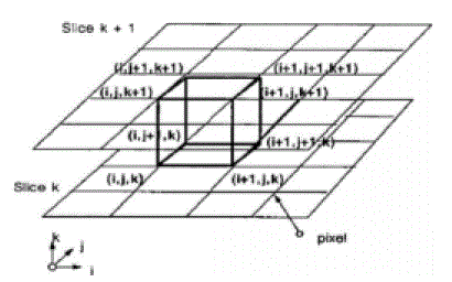
The fundamental of MC algorithm is to divide the volume data into voxels, check the voxels one by one and pick out the voxels that intersect with isosurface. Then calculate the intersection points by use of linear interpolation. Finally, connect the intersection points by a certain form according to the relative position of voxels and isosurface to form the surface, which is regarded as the approximation of the isosurface in the voxels.Relative position of voxels and isosurface [7].

There are two features in the MC algorithm:

(1) Each of the triangles contacts with some voxel.

(2) Each of the triangle-meshes extends in one sequence. In other words, there exists relativity between current one and that of the neighbour voxels in other directions (front, back, left, above, down) [2].

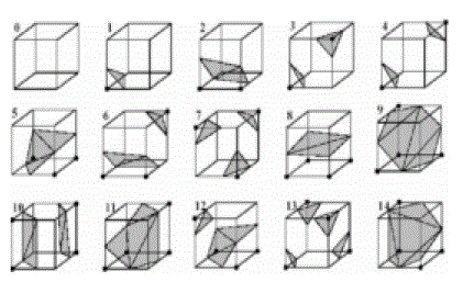
As each voxel has 8 vertices and each of them has two states of inside or outside the isosurface, we have at least 2⁸ = 256 mesh models of the isosurface. The number of the mesh models can be reduced to 15 in view of the symmetry [2], as shown in Figure 3.

The normal of the voxel can be replaced by the gradient of the central point of the voxel, which is obtained through central difference method shown as formula (5), (6), (7) and (8). The original 3D data sets are used for computing normal, which can ensure the smooth of the reconstructed image. [2]

(5)

(6)

(7)

(8)

VOLUME ROTATION METHODS

Visualization by only implementing surface reconstruction methods is not flexible to render and display any desired viewing angles. It is necessary to depict any viewing angles of the 3D object in order to provide better understanding on the nature of the object as well as identify the location of abnormalities in the structures of the object more accurately and efficiently [9].There are two approaches to visualize the data in different viewing angles, either change the direction of rays or rotate the volume of dataset.

A. Euclidean Transformation

Euclidean transformation is the most commonly used transformation method. This transformation consists of translation, rotation or reflection. In this project, only volume rotation was implemented. The transformation involves a fairly simple trigonometric calculation to obtain a transformation matrix for a rotation about the coordinate axes. It preserves length angle measure and the shape of a geometric object will not change. In other words, the geometry of the transformed object remains unchanged. Most viewing transforms are rigid body transformation. The transformation cannot rotate the volume in real time because it involves complex computations of trigonometry functions. Equations (9), (10) and (11) show rotation about the z-axis by an angle θ.

(9)

(10)

(11)

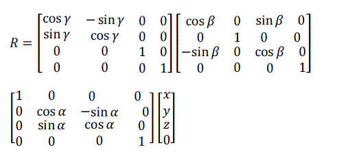
In volume rotation, there are three degrees of freedom corresponding to the ability to rotate independently about the three coordinate axes [9]. Equation (12) shows the construction of the volume rotation as a product of individual rotation about the three axes.

(12)

Equation (12) can be written in matrix form as:

(13)

Where α, β and γ are the rotation angles in x, y and z directions, respectively.

B. Shear Transformation

The effect of a shear transformation looks like pushing a geometric object in a direction that is parallel to a coordinate plane in 3D or coordinate axis in 2D. A rotation in the plane can be expressed as a composition of three shears along two orthogonal axes. Fig 4 illustrates 2D rotation achieved by three shears [9].

A rotation in the plane by an angle ψ ≠ ? can be written as a composition of three shears, each along one of the two axes and across the other, namely

(14)

Equation (14) can be written in matrix form as:

(15)

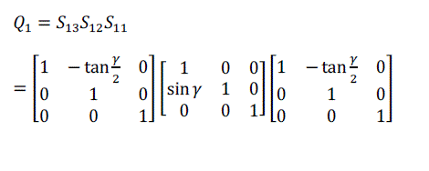
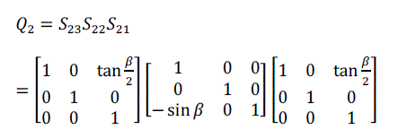
For volume rotation, one can apply decomposition of Equation (15) separately to three rotations along x, y and z axis respectively, obtaining the shear products as Equation (16), (17) and (18) in matrix form. As a result, Q = R(γ, β, α) can be written as the product of nine shears as Equation (19).

(16)

(17)

(18)

(19)

This is how Shear Transformation can be carried out.

CONCLUSION

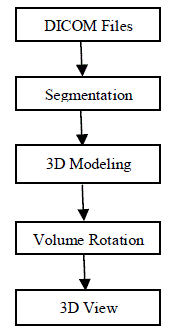
In this paper, an accurate surface reconstruction method of medical image is proposed. In this algorithm, suitable segmentation methods are used to abstract the region for 3D modeling using Marching Cube. Marching cubes, an efficient algorithm for 3D surface construction, complements 2D CT data by giving physicians 3D views of the anatomy. The algorithm uses a case table of edge intersections to describe how a surface cuts through each cube in a 3D data set. Using volume rotation method we can view this 3D model from different angle.

However, there are still some points for future study. Surface rendering and volume rendering can be integrated. The module of image fusion could be added after the module of segmentation, for example, the data of the CT slices can be reconstructed after the fusion with PET images, leading the therapy and diagnosis more effective.

Figures at a glance


Figure 1	Figure 2	Figure 3	Figure 4

References

T.Senthil Kumar, Anupa Vijai “3D Reconstruction of Face from 2D CT Scan Images” International Conference on Communication Technologyand System Design 2011, Procedia Engineering 30 (2012) 970-977

Bin Lee, Lian-Fang Tian, Chen Ping, Hong Qiang Mo, Zong-Yuan Mao “A Fast Accurate 3D Surface Reconstruction Method Of MedicalImage Based On Modularization” Proceedings of Fourth International Conference on Machine Learnig and Cybernetics, Guangzhou, August2005, 0-7803-9091-1/05/2005 IEEE

Avnish Patel, Kinjal Mehta “3D Modeling and Rendering of 2D Medical Image” 2012, International Conference on Communication Systemsand Network Technologies, 978-0-7695-4692-6/12, 2012 IEEE

Serdar Kemal Balci “Medical Image Segmentation Using Active Contours” Image Processing, Term Project Report, June 2006, EE-574.

Tony F. Chan, Luminita A. Vese “Active Contours Without Edges” IEEE Transactions On Image Processing, Vol. 10, No. 2, February 2001.

M. Kass, A. Witkin, D. Terzopoulos, ” Snakes: Active contour models,” International Journal of Computer Vision,vol. 1, pp. 321-331, 1988.

William E. Lorenson, Harvey E. Cline “Marching Cubes: A High Resolution 3d Surface Construction Algorithm” Computer Graphics, Volume21, Number 4, July 1987.

Jun Xiao, Miao Yu, Ningyu Jia “An Improved MC Algorithm Applied in Medical Image Reconstruction” College of Information Science andEngineering, Northeastern University, China, 978-1-4244-1734-6/08/2008 IEEE

Thean Wui Ooi, Haidi Ibrahim, Kenny Kal Vin Toh “Implementation of Several Rendering and Volume Rotation Methods for VolumeRendering of 3D Medical Dataset” 2008 IEEE Conference on Innovative Technologies in Intelligent Systems and Industrial ApplicationsMultimedia University, Cyberjaya, Malaysia, 12-13 July 2008.