A Fusion Sorting Technique Using Multithreading Approach

Abstract

Sorting is one of the most common operations performed by computers especially in database applications where uploading is done by sorting transactions and merging them with a master file. People prefer relevant data to be sorted before wading through various pages of data. It is ubiquitous in engineering applications in all disciplines. There is only one basic strategy of sorting but the variations are of a great number. Algorithms like bubble sort remain favorite of people especially beginners as they first strike their mind when they sort not keeping in mind the factors such as time complexity which will be discussed extensively in our paper. Here we have discussed a few sorting algorithms with their complexities and have proposed a fusion method of sorting which uses the popular bubble sort in combination with merge sort using the multi-threading approach.

Keywords

sorting techniques, sorting methods, bubble sort, merge sort, time complexity, space complexity

INTRODUCTION

Sorting is the process of placing elements from a collection in some kind of order. For example, a list of words could be sorted alphabetically or by length. A list of cities could be sorted by population, by area, or by zip code. There are many, many sorting algorithms that have been developed and analyzed. This suggests that sorting is an important area of study in computer science. Sorting a large number of items can take a substantial amount of computing resources. Like searching, the efficiency of a sorting algorithm is related to the number of items being processed. For small collections, a complex sorting method may be more trouble than it is worth. The overhead may be too high. On the other hand, for larger collections, we want to take advantage of as many improvements as possible. In this paper we will discuss several sorting techniques and compare them with respect to their running time and space.

Before getting into specific algorithms, we should think about the operations that can be used to analyze a sorting process. First, it will be necessary to compare two values to see which is smaller (or larger). In order to sort a collection, it will be necessary to have some systematic way to compare values to see if they are out of order. The total number of comparisons will be the most common way to measure a sort procedure. Second, when values are not in the correct position with respect to one another, it may be necessary to exchange them. This exchange is a costly operation and the total number of exchanges will also be important for evaluating the overall efficiency of the algorithm.

We have further proposed a fusion method which can be used as an internal as well as an external sorting technique. This method uses the multithreading approach. A multithreaded program makes optimal use of resources, more so when there are multiple processors in such a way that a single task is divided into multiple parts or sections which in turn execute concurrently. In this way the resources are handled very efficiently.

The actual essence of multitasking is when multiple processes share common processing resources such as a CPU. Multithreading extends the idea of multitasking into applications where you can subdivide specific operations within a single application into individual threads. Each of the threads can run in parallel. The OS divides processing time not only among different applications, but also among each thread within an application [1].

THE BUBBLE SORT

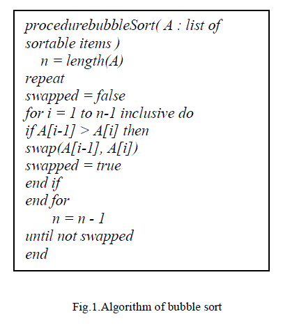
Bubble sort, sometimes referred to as sinking sort, is a simple sorting algorithm that works by repeatedly stepping through the list to be sorted, comparing each pair of adjacent items and swapping them if they are in the wrong order. The pass through the list is repeated until no swaps are needed, which indicates that the list is sorted. The algorithm gets its name from the way smaller elements "bubble" to the top of the list. Because it only uses comparisons to operate on elements, it is a comparison sort. Although the algorithm is simple, it is too slow for practical use. Example of bubble sort:

6 3 12 7 4 5 11 9 (unsorted list)

3 6 12 7 4 5 11 9

3 6 7 12 4 5 11 9

3 6 7 4 12 5 11 9

3 67 4 5 12 11 9

3 6 7 4 5 1112 9

3 6 7 4 5 11 9 12 (The largest no. bubbled to the end after inner loop executes for one value of outer loop) In this way after execution of each value of outer loop, the next largest value bubbles down, till the list is sorted.

3 64 5 7 9 11 12

3 4 5 6 7 9 11 12

Repeat the same till no more swaps are possible. After every pass the next largest number bubbles down.

3 6 4 7 5 9 11 12

3 4 6 5 7 9 11 12

3 4 5 6 7 9 11 12

3 4 5 6 7 9 11 12 (No swaps required so list is sorted)

A. Properties of Bubble Sort:

The properties of this sorting technique as per the time and space complexities are:

• Stable

• O(1) extra space

• O(n2) comparisons and swaps

• Adaptive: O(n) when nearly sorted

The algorithm itself is as shown in Fig. 1.

THE INSERTION SORT

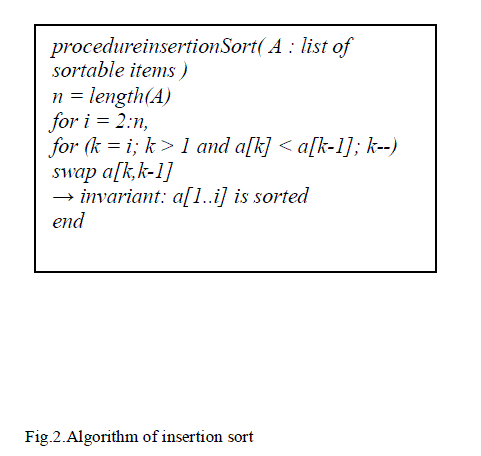
In each iteration of insertion sort, one element from the inputted list is removed and then inserted in its correct position in the sorted list. This process continues until no input elements remain. The final list in insertion sort is built one element at a time. Insertion sort is of choice either when the problem is almost sorted or is of small size.

The simplest worst case input is an array sorted in reverse order. The set of all worst case inputs consists of all arrays where each element is the smallest or second-smallest of the elements before it. In these cases every iteration of the inner loop will scan and shift the entire sorted subsection of the array before inserting the next element.

Typical example of insertion sort is sorting playing cards manually in a particular order. The average case of insertion sort is quadratic which is why it is impractical for sorting large arrays. However insertion sort is even faster than quicksort for sorting small arrays.

Example of insertion sort:

6 3 12 7 4 5 11 9 (unsorted list)

Take one element at a time –

6

3 6

3 6 12

3 6 7 12 (like picking up cards one by one and inserting in the right position)

3 4 6 7 12

3 4 5 6 7 12

3 4 5 6 7 11 12

3 4 5 6 7 9 11 12 (sorted list)

A. Properties of Insertion Sort:

The properties of this sorting technique as per the time and space complexities are:

• Stable

• O(1) extra space

• O(n2) comparisons and swaps

• Adaptive: O(n) time when nearly sorted

• Very low overhead

The algorithm itself is as shown in Fig. 2.

THE SELECTION SORT

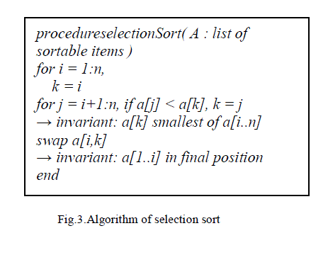
The idea of selection sort is rather simple: we repeatedly find the next largest (or smallest) element in the array and move it to its final position in the sorted array. Assume that we wish to sort the array in increasing order, i.e. the smallest element at the beginning of the array and the largest element at the end. We begin by selecting the largest element and moving it to the highest index position.

Selecting the lowest element in selection sort requires scanning n elements and n-1 comparisons and swapping it to the lowest position. Selecting the second element requires scanning n-1 elements and so on. Each of these scans requires one swap for n − 1 elements (the final element is already in place).

While selection sort is preferable over insertion sort in terms of number of writes (O(n) swaps to O(n2 ) swaps) but is greatly outperformed by divide and conquer algorithms such as merge sort. But both insertion and selection sorts are typically faster for small arrays.

Example of selection sort:

6 3 12 7 4 5 11 9 (unsorted list)

3 6 12 7 4 5 11 9 (Find the smallest and place it at its right position after swapping – 3 swapped with 6)

3 4 12 7 6 5 11 9 (4 swapped with 6)

3 4 5 7 6 12 11 9 ( 5 swapped with 12)

3 4 5 6 7 12 11 9 (6 swapped with 7)

3 4 5 6 7 9 11 12 (9 swapped with 12)

A. Properties of Selection Sort:

The properties of this sorting technique as per the time and space complexities are:

• Not stable

• O(1) extra space

• O(n2) comparisons

• O(n) swaps

• Not adaptive

The algorithm itself is as shown in Fig. 3.

THE QUICK SORT

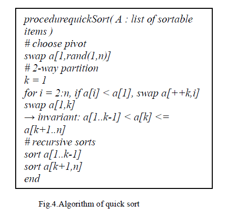
Quick sort is a divide and conquer algorithm. It divides a large array into two sub arrays and then sorts the subsequent two arrays recursively. The steps of quick sort are:

1. Pick an element, called a pivot, from the array.

2. Reorder the array so that all elements with values less than the pivot come before the pivot, while all elements with values greater than the pivot come after it (equal values can go either way). After this partitioning, the pivot is in its final position. This is called the partition operation.

3. Recursively apply the above steps to the sub-array of elements with smaller values and separately to the subarray of elements with greater values.

Space required by quick sort is very less. Only O(n log n) additional space is required. Quick sort is a very unstable sorting technique. So it changes the occurrence of two similar elements in the list while sorting.

Example of quick sort:

6 3 12 7 4 5 11 9 (unsorted list)

6 3 12 7 4 5 11 9 (Find no. smaller than 6 from Right to Left and swap - 6 and 5 to be swapped)

5 312 7 4 6 11 9 (Find no. greater than 6 from Left to Right and swap - 6 and 12 to be swapped)

5 3 6 7 4 12 11 9 (Repeat R to L - 6 and 4 to be swapped)

5 3 4 7 6 12 11 9 (Repeat L to R – 6 and 7 to be swapped)

5 3 4 6 7 12 11 9 (6 is at its right position and 6 is the pivot)

Repeat this for sublist on left of 6 and for sublist on right of 6. Keep on doing this till list is sorted.

A. Properties of Quick Sort:

The properties of this sorting technique as per the time and space complexities are:

• Not stable

• O(1) extra space

• O(n2) comparisons

• O(n) swaps

• Not adaptive

The algorithm itself is as shown in Fig. 4.

THE HEAP SORT

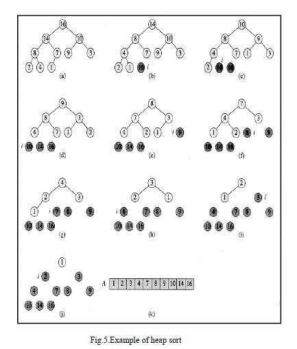
The heap data structure is an array object that can be viewed as a complete binary tree. In the first step the heap is built. Each node of the tree corresponds to an element of the array that stores the value in the node. The complete binary tree maps the binary tree structure into the array indices; each array index represents a node; the indexes of the node’s parent, left child branch, or right child branch are simple expressions [8]. In the second step, a sorted array is created by repeatedly removing the largest element from the heap (the root of the heap), and inserting it into the array. The heap is updated after each removal to maintain the heap. Once all objects have been removed from the heap, the result is a sorted array.

Heapsort can be performed in place. The array can be split into two parts, the sorted array and the heap. The heapSort procedure takes time O(n log n), since the call to create the heap takes time O(n) and each of the n - 1 calls to delete the root and maintain the heap takes time O(log n). The given sequence of numbers is first converted in the form of a binary heap. Example of the Heap Sort is shown in Fig. 5.

A. Properties of Heap Sort:

The properties of this sorting technique as per the time and space complexities are:

• Not stable

• O(1) extra space

• O(n log n) time

• Not really adaptive

• Does not require random access to data

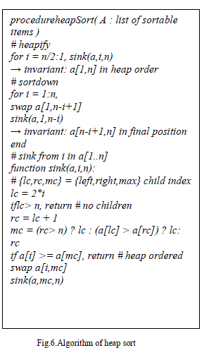
The algorithm itself is as shown in Fig. 6.

THE MERGE SORT

Merge sort is also based on the divide and conquer paradigm. Its worst-case running time has a lower order of growth than insertion sort. To sort A[p .. r]:

1. Divide Step

If a given array A has zero or one element, simply return; it is already sorted. Otherwise, split A[p .. r] into two subarrays A[p .. q] and A[q + 1 .. r], each containing about half of the elements of A[p .. r]. That is, q is the halfway point of A[p .. r].

2. Conquer Step

Conquer by recursively sorting the two subarrays A[p .. q] and A[q + 1 .. r].

3. Combine Step

Combine the elements back in A[p .. r] by merging the two sorted subarrays A[p .. q] and A[q + 1 .. r] into a sorted sequence. To accomplish this step, we will define a procedure MERGE (A, p, q, r).

Example of merge sort:

6 3 12 7 4 5 11 9 (unsorted list)

6 312 74 511 9 (divide the sublists in two each)

3 67 124 59 11 (sort the sublists)

3 6 7 124 5 9 11 (merge the two consecutive sublists two at a time)

3 4 5 6 7 9 11 12(go on merging till one list remains)

A. Properties of Merge Sort:

The properties of this sorting technique as per the time and space complexities are:

• Stable

• O(n) extra space for arrays (as shown)

• O(log n) extra space for linked lists

• O(n log n) time

• Not adaptive

• Does not require random access to data

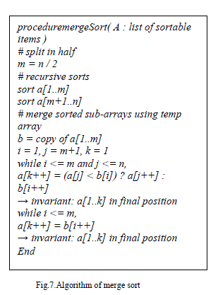
The algorithm itself is as shown in Fig. 7.

THE RADIX SORT

The Radix Sort is useful for large arrays where numbers are relatively small compared to the size of the array. This method is a variant of the bucket sorting method.

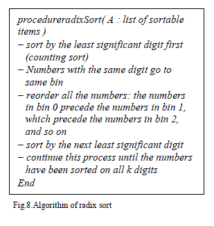
This sorting is applicable only when the values are integer numerals in some base. Over here depending on maximum number of digits in the given list, the numbers of radix or buckets are created. We sort on each digit of the numerals starting from the least significant one. We continue sorting in this way progressively towards the most significant one.

After each distribution, we regroup the items anew taking care to preserve their order from the previous distribution. When the last regrouping is over the items are sorted. [5]

A. Properties of Radix Sort:

The properties of this sorting technique as per the time and space complexities are:

• Stable

• O(n + N) extra space for arrays

• O(nk) time (k is number of digits in the largest numeral)

• Not adaptive

The algorithm itself is as shown in Fig. 8.

Example of radix sort:[6, 7]

Original, unsorted list:

170, 45, 75, 90, 802, 2, 24, 66

Sorting by least significant digit (1s place) gives:

170, 90, 802, 2, 24, 45, 75, 66

(Notice that we keep 802 before 2, because 802 occurred before 2 in the original list, and similarly for pairs 170 & 90 and 45 & 75.)

Sorting by next digit (10s place) gives:

802, 2, 24, 45, 66, 170, 75, 90

Notice that 802 again comes before 2 as 802 comes before 2 in the previous list.

Sorting by most significant digit (100s place) gives:

2, 24, 45, 66, 75, 90, 170, 802

This is the final sorted list.

THE PROPOSED FUSIONSORT

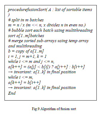
We have designed a new method which can be used when the number of items to be sorted is very large. It can be used as an external sorting method. This method involves the concept of multithreading.

Multithreading is the ability of a program or an operating system process to manage its use by more than one user at a time and to even manage multiple requests by the same user without having to have multiple copies of the program running in the computer. Central processing units have hardware support to efficiently execute multiple threads. Assume that the total number of items are N. Divide the items in M groups in such a way that M is an even number. This means that our items are now divided in M batches and the size of each batch is more or less same. It is possible that all groups/batch may not have the same number of items as N is not necessarily an even number.

This method will work in two phases:

Phase 1:

Using multithreading, sort each group simultaneously using the bubblesort method. Since each group size is more or less same, the time taken to sort each group would be same.

Phase 2:

Take as input the sorted groups two at a time and using merge sort start combining the groups. This time also the concept of multithreading can be used so that the merging will be fast and will reduce the time complexity. Keep on merging the groups till the final sorted items are derived.

In the first phase, instead of bubble sort we can take any other sorting technique. Here since the items are divided in small groups and then sorted in the first phase the time complexity is O (1) assuming each group size is << N.

In the second phase again the merging takes place concurrently so the time complexity would be O (n log n) as in merge sort. So the final complexity is O (n log n).The example of this method would be similar to the one show in bubble sort and merge sort with the only change being that the sorting takes place for each batch simultaneously.

Example of fusion sort:

6 3 12 7 4 5 11 9 (unsorted list)

6 3 12 74 5 11 9 (divide the sublists in M batches e.g. 2)

3 6 7 12 4 5 9 11 (sort the sublistssimultaneouly)

3 6 7 12 4 5 9 11 (merge the Msublistssimultaneouly)

A. Properties of Fusion Sort:

The properties of this sorting technique as per the time and space complexities are:

• Stable

• O(n) extra space for arrays

• O(n log n) time

• Not adaptive

• external sorting technique

The algorithm itself is as shown in Fig. 9.

THE COMPARATIVE STUDY

The comparative study between the different sorting techniques and the proposed new technique is as shown in Tab. 1 below. The table shows each sorting method discussed above as well as the proposed Fusion Sort technique with a comparison of the time complexities best, average and worst cases and the space complexity.

CONCLUSION

As mentioned before, sorting is one of the most common operations performed by computers and programmers in varied areas of computer science and engineering. Depending on the type of application, size of data and nature of data the most appropriate sorting algorithm can be chosen. Nowadays when space and processor speed is not required to be compromised, the method proposed by us would prove to be a very good option for large data size.

Still this area remains to be one of the most enormously implemented and extensively sought comparative studies for computer professionals. There can be no one final method of sorting which can cater to all requirements universally.

Tables at a glance

Table 1

Figures at a glance

Figure 1 Figure 2 Figure 3 Figure 4 Figure 5 Figure 6 Figure 7 Figure 8 Figure 9

References

http://www.tutorialspoint.com/ Seymour Lipschutz, “Data Structures”, McGraw Hill Education (India) Private Limited, pp. 9.1-9.27, 2010. Tremblay and Sorenson, “An Intoduction to Data Structures with Applications”, McGraw Hill, pp. 538-562, 1984. R. B. Patel, “Expert Data Structures with C”,Khanna Book Publishers, pp. 595-645, 2001. P. H. Dave and H. B. Dave, “Design and Analysis of Algorithms”, Pearson, pp. 407, 2007. http://www.geeksforgeeks.org/radix-sort/ http://en.wikipedia.org/wiki/Radix_sort http://en.wikipedia.org/wiki/Heapsort