A New Approach of Performance Analysis of
Adaptive Filter Algorithm in Noise Elimination

Asaduj Jahan Jimi; Mohammad Manzurul Islam; M. F Mridha

A New Approach of Performance Analysis of Adaptive Filter Algorithm in Noise Elimination

Asaduj Jahan Jimi¹, Mohammad Manzurul Islam² and M. F Mridha³

CSE Department, Stamford University Bangladesh, Dhaka, Bangladesh
Faculty of Engineering and IT, University of Technology Sydney (UTS), Sydney, Australia
Assistant Professor, CSE, University of Asia Pacific, Dhaka, Bangladesh

Related article at Pubmed, Scholar Google

Visit for more related articles at International Journal of Advanced Research in Electrical, Electronics and Instrumentation Engineering

Abstract

Adaptive Filtering is an extreme researched topic in the present era of digital communications. When the received signal is rapidly disturbed by noise where both the received signal and noise change continuously, then arises the need for adaptive filtering. The core of the adaptive filter is the adaptive algorithm. This paper deals with elimination of noise on speech signal and data signals using four algorithms-Least Mean Square (LMS) algorithm, Normalized Least Mean Squares(NLMS) algorithm, Recursive Least Squares (RLS) and Fast Transversal Filter (FTF) algorithm with implementation in MATLAB. Comparisons of the algorithms are based on forgetting factor and tap weights of filter. The algorithms chosen for implementation provide efficient performances with less computational complexity.

Index Terms

Adaptive Filtering, adaptive algorithm, Least Mean Square (LMS), Normalized Least Mean Squares(NLMS) , Recursive Least Squares (RLS) and Fast Transversal Filter (FTF) algorithm.

INTRODUCTION

Digital signal processing (DSP) is concerned with the representation of signals by a sequence of numbers or symbols and the processing of these signals. Digital signal processing and analog signal processing are subfields of signal processing. DSP includes subfields like: audio and speech signal processing, sonar and radar signal processing, sensor array processing, spectral estimation, statistical signal processing, digital image processing, signal processing for communications, control of systems, biomedical signal processing, seismic data processing, etc. The goal of DSP is usually to measure, filter and compress continuous real-world analog signals. The first step is usually to convert the signal from an analog to a digital form, by sampling it using an analog-to-digital converter (ADC), which turns the analog signal into a stream of numbers [1]. However, often, the required output signal is another analog output signal, which requires a digital-to-analog converter (DAC). Even if this process is more complex than analog processing and has a discrete value range, the application of computational power to digital signal processing allows for many advantages over analog processing in many applications, such as error detection and correction in transmission as well as data compression. Today technologies are used for digital signal processing including more powerful general purpose microprocessors; field-programmable gate arrays (FPGAs), digital signal controllers and stream processors, among others.

LITERATURE REVIEW

The earliest work on adaptive filters may be traced back to the late 1950s, during which time a number of researchers were working independently on different applications of such filters. From this early work, the least-mean-square algorithm (LMS) [2] emerged as a simple, yet effective, algorithm for the operations of adaptive transversal filters. The LMS algorithm was devised by Widrow and Hoff in 1959 in their study of pattern-recognition scheme known as the adaptive linear element, commonly referred to in the literature as the Adaline [2, 3]. The LMS algorithm is a stochastic gradient algorithm in that it iterates each tap weight of a transversal filter in the direction of the gradient of the squared magnitude of an error signal with respect to the tap weight. Accordingly the LMS algorithm is closely related to the concept of stochastic approximation developed by Robbins and Monro (1951) in statistics for solving certain sequential parameter estimation problems. The primary difference between them is that the LMS algorithm uses a fixed-size parameter to control the correction applied to each tap weight from one iteration to the next, where as in stochastic approximation methods the step-size parameter is made inversely proportional to time n. Another stochastic gradient algorithm, closely related to the LMS algorithm, is the Recursive least square (RLS) algorithm Hayes, Monson H. (1996) [4]; the difference between them is:

1. In the LMS algorithm, the correction that is applied in updating the old estimate of the coefficient vector is based on the instantaneous sample value of the tap-input vector and the error signal. On the other hand, in the RLS algorithm the computation of this correction utilizes all the past available information.

2. The LMS algorithm requires approximately 20M iterations to converge in mean square, where M is the number of tap coefficients contained in the tapped-delay-line filter. On the other band, the RLS algorithm converges in mean square within less than 2M iterations. The rate of convergence of the RLS algorithm is therefore, in general, faster than that of the LMS algorithm by an order of magnitude.

3. Unlike the LMS algorithm, there are no approximations made in the derivation of the RLS algorithm. Accordingly, as the number of iterations approaches infinity, the least-squares estimate of the coefficient vector approaches the optimum Wiener value, and correspondingly, the mean-square error approaches the minimum value possible. In other words, the RLS algorithm, in theory, exhibits zero maladjustment. On the other hand, the LMS algorithm always exhibits a nonzero maladjustment; however, this maladjustment may be made arbitrarily small by using a sufficiently small step-size parameter μ.

ADAPTIVE ALGORITHMS

A) Least Mean Square adaptation Algorithm (LMS)

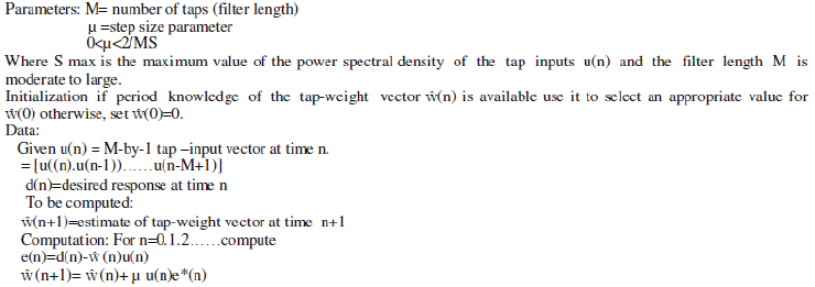
LMS incorporates an iterative procedure that makes successive corrections to the weight vector in the direction of the negative of the gradient vector which eventually leads to the minimum mean square error. Compared to other algorithms LMS algorithm is relatively simple; it does not require correlation function calculation nor does it require matrix inversions.

B) The Normalized LMS (NLMS) introduces a variable adaptation rate. It improves the convergence speed in a non-static environment. In another version, the Newton LMS, the weight update equation includes whitening in order to achieve a single mode of convergence. For long adaptation processes the Block LMS is used to make the LMS faster. In block LMS, the input signal is divided into blocks and weights are updated block wise. A simple version of LMS is called the Sign LMS. It uses the sign of the error to update the weights. Also, LMS is not a blind algorithm i.e. it requires a priori information for the reference signal.

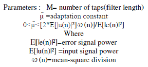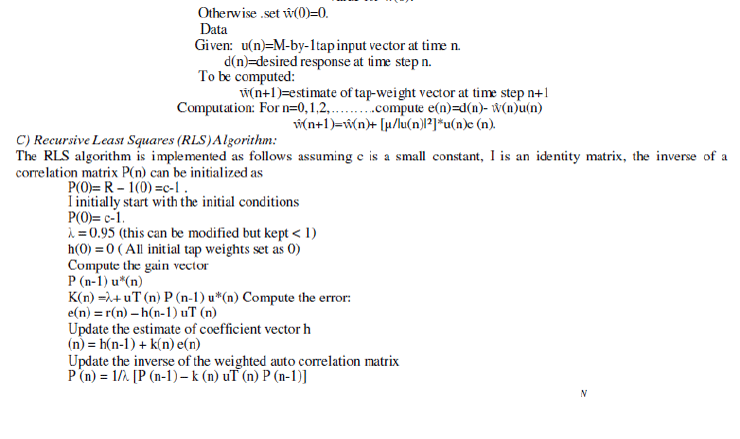
Initialization: If prior knowledge about the tap-weight vector w(n) is available, use the knowledge to select an appropriate value for Ãâ¦ÃÂµ(0).

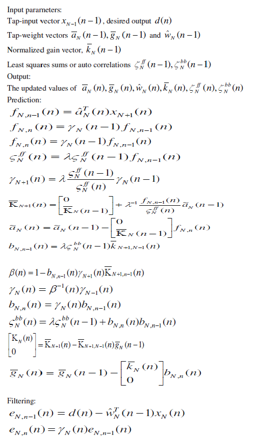
D) Fast Transversal Filter (FTF) Algorithm: The RLS algorithm and square root RLS algorithm have a computational complexity that increases as the square of M, where M is the number of adjustable weights (number of degrees of freedom) in the algorithm. The FTF algorithm is summarized below by collecting together the relevant equations.

SIMULATION AND PERFORMANCE ANALYSIS

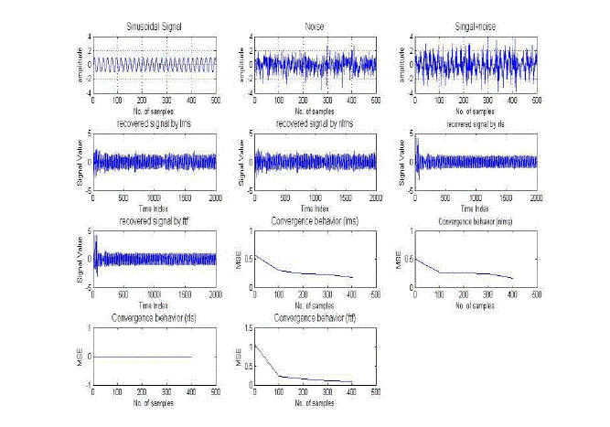
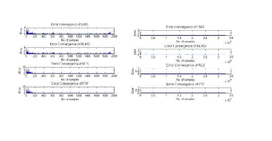
In this paper, simulation based on two different types of signals mixed with various types of noise. Signals are sinusoidal and speech signal. Each signal has been subjected to some noise. Then the convergence behaviours of the LMS, NLMS, RLS, and FTF algorithms for these signals have been analysed. The objective of this section is to show the general noise elimination characteristics of these four algorithms Detail analysis and comparison are shown in subsequent sections. Figure 1 consists of 11 graphs the top three graphs show original signal, noisy signal and original signal’s state after mixing of noise. The middle four graphs show the recovered signals obtained by the LMS, NLMS, RLS and FTF algorithms respectively. The lowermost four graphs show the error convergence of the LMS, NLMS, RLS and FTF algorithm.

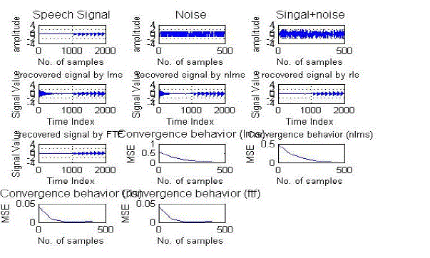
Figure 2 consist of 11 graphs. The top three graphs show original signal, n y g l r g l g l’ e f er mixing of noise. The middle four graphs show the recovered signals obtained by the LMS,NLMS,RLS and FTF algorithms respectively. The lowermost four graphs show the error convergence of the LMS,NLMS,RLS and FTF algorithm respectively.

A) Effect of filter length on the performance of the algorithms

Filter length refers to the number of coefficients of the filter. This number is significant in case of performance analysis. In this thesis, noises are cancelled by varying the filter length while all other parameters keep in unchanged.

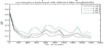
I) Effect of filter length on LMS

• For filter length = 10, around 100th sample, MSE converges to zero

• For filter length = 16, around 110th sample, MSE converges to zero.

• For filter length = 20, around 120th sample, MSE converges to zero.

• For filter length = 32, around 130th sample, MSE converges to zero.

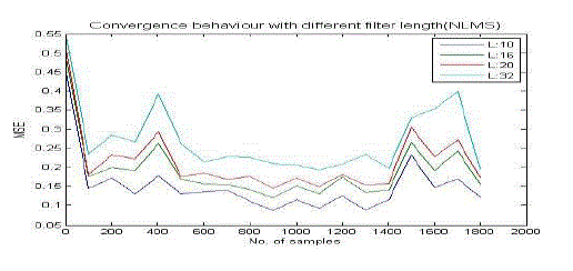
II) Effect of filter length on NLMS

• For filter length = 10, around 100th sample, MSE converges to zero

• For filter length = 16, around 110th sample, MSE converges to zero.

• For filter length = 20, around 120th sample, MSE converges to zero.

• For filter length = 32, around 130th sample, MSE converges to zero.

III) Effect of filter length on RLS

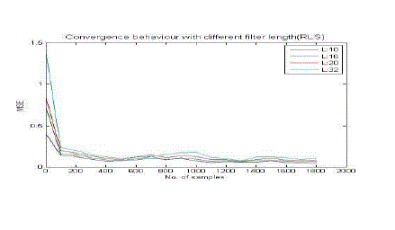
For filter length = 10, around 15th sample, MSE converges to zero

For filter length = 16, around 30th sample, MSE converges to zero.

For filter length = 20, around 40th sample, MSE converges to zero.

For filter length = 32, around 50th sample, MSE converges to zero.

IV) Effect of filter length on FTF

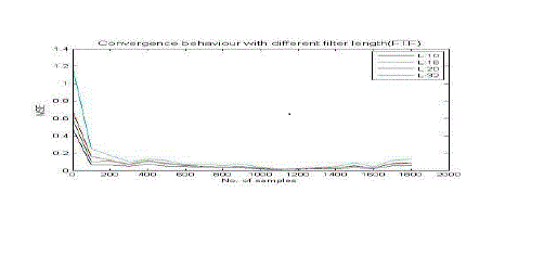
For filter length = 10, around 15th sample, MSE converges to zero

For filter length = 16, around 30th sample, MSE converges to zero.

For filter length = 20, around 40th sample, MSE converges to zero.

For filter length = 32, around 50th sample, MSE converges to zero.

From the simulation results, it is clear that, if the filter length is increased, then number of iterations of the adaptive algorithms increase to converge the MSE towards zero.

Hence, the simulation results reveal that if the number of iterations is calculated, then it is observed that, adaptive filter with small filter length performs noise cancellation faster than higher filter length. So filter length 10 is the best choice. Forgetting factor or exponential weighting factor is an important parameter of RLS and FTF algorithms and it controls the stability and the rate of convergence. Generally it is a constant close to, but smaller than one. In the ordinary method of least square λ=1. When λ<1, the weighting factor gives more weight to the recent samples of the error estimates (and thus the recent samples of the observed data) compared with the old ones In other words, the choice of λ<1 results in a scheme that puts more emphasis on the recent samples of the observed data and tends to forget the past.

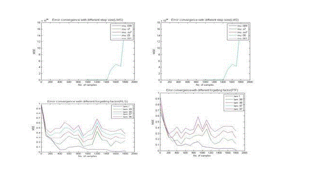
Similarly, the step size parameter of the LMS and NLMS algorithms controls the stability and the rate of convergence. If the step size parameter is chosen to be very small, then the algorithm goes close to the solution but it takes more time to converge. On the other hand, if the step size parameter is chosen to be large, then the algorithm converges quickly but may be diverged. So it is very essential and critical to select the perfect step size parameter. In this section it is tried to find out the appropriate step size and forgetting factor parameter for the algorithms. The performance is actually measured by MSE (mean square error) of the output error. The smaller MSE, the more it can ensure the certification for better adaptation.

The convergence analysis of the RLS and FTF algorithms presented in this section assumes that the exponential weighting factor is unit; MSE performs faster convergence than other values.

From the above observation it is found that, the best value of the forgetting factor parameter of the RLS,FTF algorithms is one, and the Step size parameter value of the NLMS algorithms is .009 can perform the best for converging, neither greater value from it nor less value performs well.

B) Comparison of the Performances of the LMS, NLMS, RLS, and FTF Algorithms:

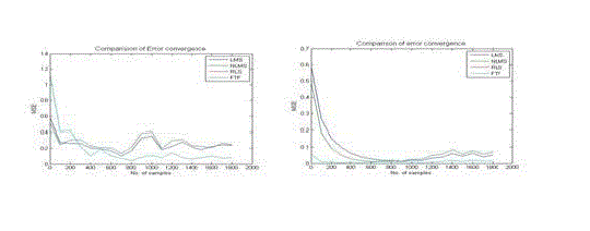
Some noise cancellation simulations and some parameters (like step size, filter length, forgetting factor) that define the characteristics of the adaptive algorithms have been presented in the above section. This section focuses on the comparison of four algorithms by analyzing error cancellation capability of these four algorithms using the best values of those parameters obtained from the previous simulations. Now, the comparison of the performance of these algorithms in the context of convergence behavior, convergence time, correlation coefficient and signal to noise ratio (SNR) will be attempted to done.

From the simulation results, it is clear that, In the case of sinusoidal signal (mixed with random noise), RLS and FTF algorithms perform better than (LMS, NLMS) and they almost show same convergence behaviour. But, LMS and NLMS’s performance is not satisfactory in this case. LMS, NLMS performs the best in the case of speech signal when it is mixed with random noise. Hence worth, FTF and RLS perform here at the same level in this situation. But FTF algorithm is complex but RLS algorithm is simple, for this RLS is better than FTF.

CONCLUSION

The components of adaptive noise eliminator were generated by computer simulation using MATLAB. The performance of the adaptive algorithms in noise elimination was analysed using various measurement criteria. Different types of inputs and noises have been employed for the analysis. The analysis was revealed that, for the LMS, NLMS, RLS and FTF algorithms, the increase in filter length results in increased MSE and increased convergence time. In t h i s paper for making a comparison among these algorithms, noise cancellation performance, convergence time and making the signal to noise ratio high are analyzed. It is found in all cases that RLS has performed as medium level in cancelling noise. In some cases FTF may have taken slightly more time to converge, but its error has always dipped down below that of the RLS algorithms. In the case of convergence time LMS, NLMS algorithm shows the best performance among four algorithms. In s i g n a l s where the amp l i t u d e or f r eq uency encounters abrupt changes, the RLS and FTF algorithms show poor performance .In these cases RLS and FTF graphs show sudden rise of error whereas the LMS, NLMS remains stable to zero.

Tables at a glance


Table 1	Table 2

Figures at a glance


Figure 1	Figure 2	Figure 3	Figure 4	Figure 5

Figure 6	Figure 7	Figure 8	Figure 9

References

Haykin, S., Adaptive Filter Theory. Prentice Hall, Upper Saddle River, 3rd Edition, 1996.

A. Gilloire and M. Vetterli, “Adaptive Filtering in Subbands with Critical Sampling: Analysis, Experiments and Applications toAcoustic Echo Cancellation”. IEEE Trans. Signal Processing, vol. SP-40, no. 8, pp. 1862-1875, Aug. 1992.

J. J. Shynk, “Frequency-Domain and M ultirate Adaptive Filtering”. IEEE Signal Processing Magazine, pp. 14-37, Jan. 1992.

S. Weiss, “On Adaptive Filtering in Oversampled Sub-bands”, PhD. Thesis, Signal Processing Division, University of Strathclyde,Glasgow, May1998.

R. Brennan and T. Schneider, “Filterbank Structure and Method for Filtering and Separating an Information Signal into DifferentBands, Particularly for Audio Signal in Hearing Aids”. United States Patent6,236,731. WO 98/47313. April 16, 1997

R. Brennan and T. Schneider, “A Flexible Filterbank Structure for Extensive Signal Manipulations in Digital Hearing Aids”, Proc. IEEE Int.Symp. Circuits and Systems, pp.569-572, 1998.

Hayes, M., Statistical Digital Signal Processing and Modelling, John Wiley & Sons, Inc., New York, 1996.

S. A. D. Prasetyowati, A. Susanto, T. S. Widodo, J. E. Istiyanto, “Adaptive LMS noise cancellation of wideband vehicle’s noise signals”,Proc of InternationalConference on Green Computing ICGC 2010.2010.

E. Firmansyah, U. D. At mojo,“ECG signal preprocessing using LabView : LMS based adaptive filter for powerline interference cancellation”,Proceedings of International Conference on InformationTechnology and Electrical Engineering ICITEE 2011.

U. D. Atmojo, “Steepest descent least mean square algorithm (LMS) based adaptive filter for noise cancellation in speech signals”, Proc ofSouth East Asian Mathematical Society-GadjahMadaUniversityInternational Conference on Mathematics and Its Applications 2011

Ying He, et. al. “ The Applications and Si mulation of Adaptive Filter in Noise Canceling”, 2008 international Conference on ComputerScience and Soft ware Engineering, 2008, Vol.4, Page(s): 1 – 4.

Paulo S.R. Diniz, “Adaptive Filtering: Algorithms and Practical Implemetation ” ,ISBN 978-0-387-31274-3, Kluwer AcademicPublisher © 2008 Springer Science+Business Media, LLC, pp.77-195.

AbhishekTandon, M. Omair Ahmad, “An efficient, low-complexity, normalized LMS algorithm for echo cancellation” The 2nd AnnualIEEE Northeast Workshop on Circuits and Systems, 2004. NEWCAS 2004, Page(s): 161 – 164.

Sanaullah Khan, M.Arif and T.Majeed, “Comparison of LMS, RLS and Notch Based Adaptive Algorithms for Noise Cancellation of a typicalIndustrial Workroom”, 8th International MultitopicConference, 2004, Page(s): 169 – 173.

Yuu-Seng Lau, Zahir M. Hussian and Richard Harris, “Performance of Adaptive Filtering Algorithms: A Comparative Study”, AustralianTelecommunications, Networks and Applications Conference (ATNAC), Melbourne, 2003.