Adeniran Adefemi T1*, Ojo J. F.2 and Olilima J. O1
1Department of Mathematical Sciences, Augustine University Ilara-Epe, Nigeria
2Department of Statistics, University of Ibadan, Ibadan, Nigeria
Received Date:20/10/2018; Accepted Date: 05/11/2018; Published Date: 12/11/2018
Visit for more related articles at Research & Reviews: Journal of Statistics and Mathematical Sciences
This paper presents concepts of Bernoulli distribution, and how it can be used as an approximation of Binomial, Poisson and Gaussian distributions with different approach from earlier existing literatures. Due to discrete nature of the random variable X, a more appropriate method of Principle of Mathematical Induction (PMI) is used as an alternative approach to limiting behavior of binomial random variable. The study proved de'Moivres Laplace theorem (convergence of binomial distribution to Gaussian distribution) to all values of p such that p p ≠ 0 and p ≠ 1 using a direct approach which opposes the popular and most widely used indirect method of moment generating function.
Bernoulli distribution, binomial distribution, Poisson distribution, Gaussian distribution, Principle of Mathematical Induction, convergence, moment generating function. AMS subject classication: 60B10, 60E05, 60F25
If X is a random variable, the function f(x) whose value is P[X=x] for each value x in the range of X is called probability distribution [1]. There are various Probability distributions used in Sciences, Engineering and Social Sciences. They are numerous to the extent that there is no single literature that can give their comprehensive list. Bernoulli distribution is one of the simplest probability distributions in literature. An experiment consisting of only two mutually exclusive possible outcomes, success or failure, male or female, life or death, defective or non-defective, present or absent is called a Bernoulli trial [1-3]. These Independent trials having a common success of probability p were first studied by the Swiss mathematician, Jacques Bernoulli in his book Ars Conjectandi, published by his nephew Nicholas eight years after his death in 1713 [2,4-8].
Definition 1.1 (The Bernoulli Distribution)
If X is a random variable that takes on the value 1 when the Bernoulli trial is a success (with probability of success p є (0; 1)) and the value 0 when the Bernoulli trial is a failure (with probability of failure q=1-p), then X is called a Bernoulli Random Variable with probability function.
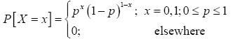 (1)
(1)
The function (1), where 0 < p < 1 and p+q=1, is called the Bernoulli probability function.
The distribution is rarely applied in real life situation because of its simplicity and because it has no strength of modeling a metric variable as it is restricted to whether an event occur or not with probabilities p and 1-p, respectively [9]. Despite this limitation, Bernoulli distribution turns (converge) to many compound and widely used robust distributions; n-Bernoulli distribution is binomial, limiting-value of binomial distribution gives Poisson distribution, binomial distribution under certain conditions yields Gaussian distribution and so on [1].
Convergence of a particular probability distribution to another and other related concepts such as limiting value of probability function or proofing of central limit theorem and law of large number had been thoroughly dealt with in literature by many authors [10-13]. All these studies adopted moment generating function (mgf) approach, perhaps because it is easy to tract and the mathematics involved is less rigorous. Based on their approach (mgf approach), they were able to establish the convergence with a valid evidence because of uniqueness property of the mgf which asserts that.
Definition 1.2 (Uniqueness Theorem)
Suppose FX and FY are two cumulative distribution functions (cdf 's) whose moments exist, if the mgf's exist for the r.v.'s X and Y and MX(t)=MY(t) for all t in -h<t<h, h>0, then, FX(u)=Y(u) for all u. That is, f(x)=f(y) for all u.
The limitation of this approach is that mgf does not exist for all distributions, yet the particular distribution approach normal or converge to other distribution under some specified condition(s). For example, the log normal distribution doesn't have a mgf, still it converges to normal distribution [14,15]. A standard/direct proof of this more general theorem uses the characteristic function which is defined for any distribution [10,11,13,16-19]. Opined that direct proving of convergence of a particular probability density function (pdf) to another pdf as n increasing indefinitely is rigorous, since it is based on the use of characteristic functions theory which involves complex analysis, the study of which primarily only advanced mathematics majors students and professors in colleges and universities understand. In this paper, we employed the direct approach to proof convergence of binomial distribution to Poisson and Gaussian distributions with a lucid explanation and supports our theorems with copious lemma to facilitate and enhance students understanding regardless of their mathematical background vis-a-vis their level.
The structure of the paper is as follows; we provide some useful preliminary results in section 2, these results will be used in section 3 where we give details convergence of Bernoulli to Binomial, Poisson and Gaussian distributions. Section 4 contains some concluding remarks.
In this section, we state some results that will be used in various proofs presented in section 3.
Proof 2.1 The proof of this lemma is as follows: using the binomial series expansion,  can be expressed as follows;
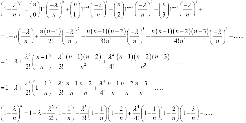
Taking limit of the preceding equation as n → ∞ gives
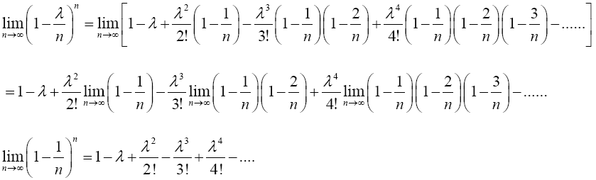
The RHS of the preceding equation is the same with Maclaurin series expansion of e-λ. Hence,
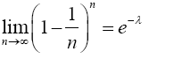 (2)
(2)
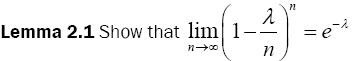
Lemma 2.2 Prove that 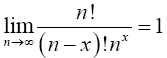
Proof 2.2
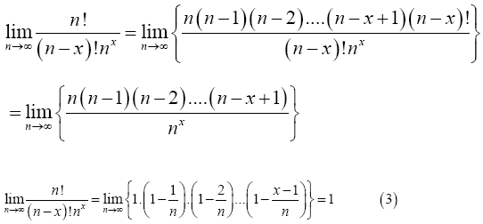
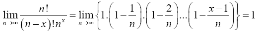 (3)
(3)
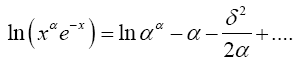
Lemma 2.3 (Stirling Approximation Principle) Given an integer α; α>0, the factorial of a large number α can be replaced with the approximation
Proof 2.3 This lemma can be derived using the integral definition of the factorial,
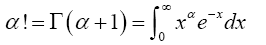 (4)
(4)
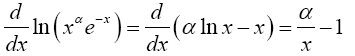
Note that the derivative of the logarithm of the integrand can be written
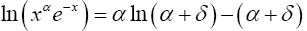
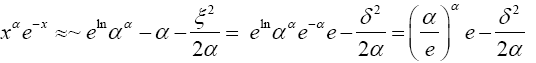
The integrand is sharply peaked with the contribution important only near x=α. Therefore, let x=α+δ where δ ≤ α, and write
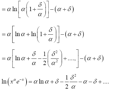
 (5)
(5)
Taking the exponential of each side of (5) gives
 (6)
(6)
Plugging (6) into the integral expression for α! that is, (4) gives
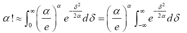 (7)
(7)
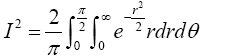
From (7), Suppose
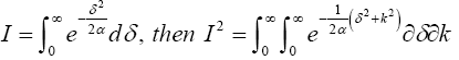
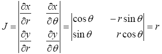
Transforming I2 from algebra to polar coordinates yields δ=ρ cos θ, k=ρ sin θ and δ2+k2=ρ2. Jacobian (J) of the transformation is
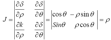
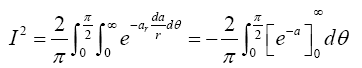
Hence,
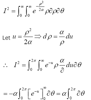
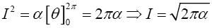
Substituting for I in (7) gives
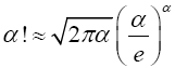 (8)
(8)
Bernoulli Probability Function to Binomial Probability Distribution
Theorem 3.1 (Convergence of bernoulli to binomial)
Suppose that the outcomes are labeled success and failure in n Bernoulli trials, and that their respective probabilities are p and q=1-p. If Sn=X is the total number of success in the n Bernoulli trials, what is the probability function of x? In other word, what is P[Sn=x] or P[X=x] for x=0,1,2……n?
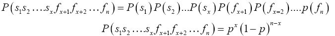
Proof 3.1 To solve this problem, let us first consider the event of obtaining a success on each of the first x Bernoulli trials followed by failures on each of the remaining n-x Bernoulli trials. To compute the probability of this event, let si denote the event of success and fi the event of failure on the ith Bernoulli trial. Then, the probability we seek is P(s1s2….sxfx+1fx+2…fn). Now, because we are dealing with repeated performances of identical experiments (Bernoulli experiments), the events s1s2….sxfx+1fx+2…fn are independent. Therefore, the probability of getting x success and n-x failures in the one specific order designated below is
 (9)
(9)
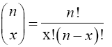
In fact, the probability of getting x success and n-x failures in any one specific order is px(1-p)n-x. Thus, the probability of getting exactly x successes in n Bernoulli trials is the number of ways in which x successes can occur among the n trials multiplied by the quantity px(1-p)n-x. Now, the number of ways in which x successes can occur among the n trials is the same as the number of distinct arrangements of n items of which x are of one kind (success) and n-x are of another kind (failure). In counting techniques, this number is the binomial coefficient
 (10)
(10)
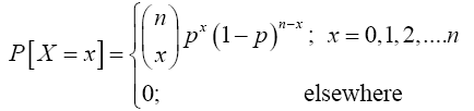
In conclusion, the probability function of Sn or X, the number of successes in n Bernoulli trials, is the product of (9) and (10) which gives
 (11)
(11)
This probability function is called the binomial probability function or the binomial probability distribution, or simply binomial distribution because of the role of the binomial coefficient in deriving the exact expression of the function. In view of its importance in probability and statistics there is a special notation for this function, as we shall see in the definition given below.
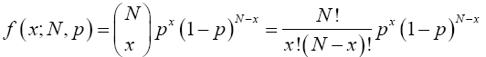
Definition 3.1 (The binomial probability function)
Let nєz+ i.e, be a positive integer, and let p and q be probabilities, with p+q=1. The function (11)
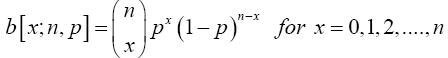
is called the binomial probability function. A random variable is said to have a binomial distribution, and is referred to as a binomial random variable, if its probability function is the binomial probability function.
Binomial Probability Function To Poisson Probability Function
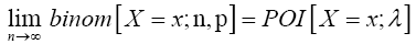
In this section, we prefer to take different approach (Principle of Mathematical Induction) to show that as n number of Bernoulli trials tends to infinity, the binomial probability binom[X=x;n,p] converges to the Poisson probability POI[X=x;λ] provided that the value of p is allowed to vary with n so that np remains equal to λ for all values of n. This is formally stated in the following theorem, which is known as Poisson's Limit Law/Theorem.
Theorem 3.2 (Poisson's limit theorem)
If p varies with n so that np=λ, where λ is a positive constant, then
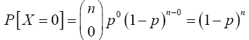
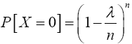
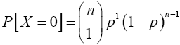
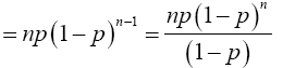
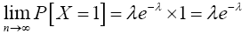
Proof 3.2 Required to show that as n → ∞, p↓0 and np → λ (a constant), one has X(n,p) →D X where X is Poisson with mean λ. Using (11), if x = 0 then
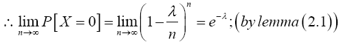
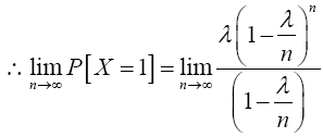
From Theorem (3.2), as n → ∞, p ↓ 0 and np → λ (a constant) implies 
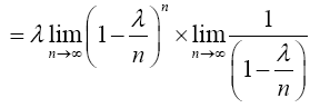
Similarly; when x=1
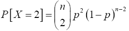
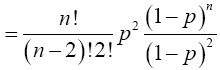
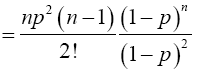
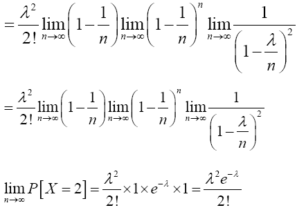
Again, when x=2,
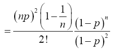
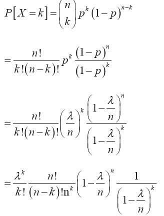
For x=k,
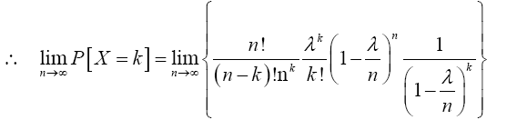
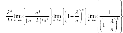
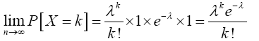
Therefore,
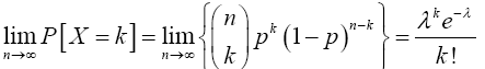 (12)
(12)
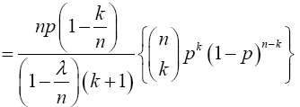
Now for x=k+1
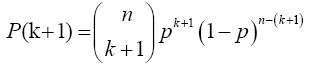
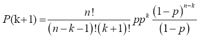
Multiplying numerator and the denominator of the preceding equation by (n-k) gives
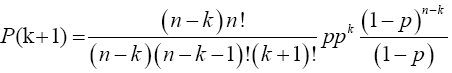
Note: As 5 X 4! = 5!, so (n-k)(n-k-1)!=(n-k)! and (k+1)!=(k+1)k!
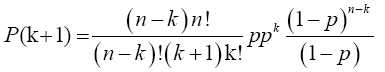
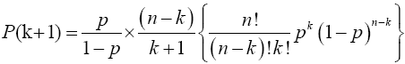
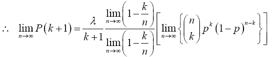
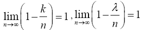 and from (12), the limit inside the square bracket is
 Hence,
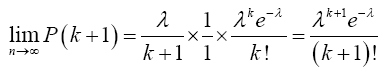 (13)
(13)
Since this is true for x=0, 1, 2,…, k and k+1, then it is true  . That is,
 (14)
(14)
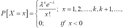
This is the required Poisson probability distribution function introduced by a French mathematician Simeon Denis Poisson (1781-1840).
Definition 3.2 (Poisson random variable) A random variable X, taking on one of the values 0, 1, 2,…, (a count of events occurring at random in regions of time or space) is said to be a Poisson random variable with parameter λ if for some λ > 0,
Equation (14) defines a probability mass function, since
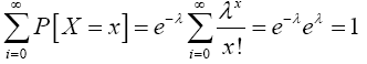 (15)
(15)
Remarks 3.1 Thus, when n is large and p is small, we have shown using Principle of Mathematical Induction approach that Poisson with parameter λ is a very good approximation to the distribution of the number of success in "n" independent Bernoulli trials.
In probability theory, de Moivre Laplace theorem asserts that under certain conditions, the probability mass function of the
random number of "successes" observed in a series of n independent Bernoulli trials, each having probability p of success, converges
to the probability density function of the normal distribution with mean np and standard deviation  as n grows
large, assuming p is not 0 or 1. The theorem appeared in the second edition of The Doctrine of Chances by Abraham de Moivre,
published in 1738 [6,17]. Although de Moivre did not use the term "Bernoulli trials", he wrote about the probability distribution of
the number of times "heads" appears when a coin is tossed 3600 times. He proved the result for p=1/2 [7,20,21]. In this paper, we
support the prove to all values of p such that p ≠ 0 and p ≠ 1.
as n grows
large, assuming p is not 0 or 1. The theorem appeared in the second edition of The Doctrine of Chances by Abraham de Moivre,
published in 1738 [6,17]. Although de Moivre did not use the term "Bernoulli trials", he wrote about the probability distribution of
the number of times "heads" appears when a coin is tossed 3600 times. He proved the result for p=1/2 [7,20,21]. In this paper, we
support the prove to all values of p such that p ≠ 0 and p ≠ 1.
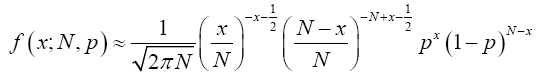
Theorem 3.3 (de Moivre's Laplace Limit Theorem) As n grows large, for x in the neighborhood of np we can approximate
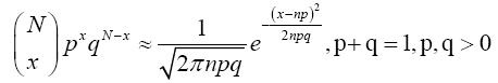 (16)
(16)
in the sense that the ratio of the left-hand side to the right-hand side converges to 1 as N → ∞, x → ∞ and p not too small and not too big.
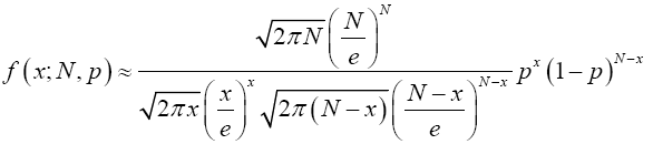
Proof 3.3 From equation (11), the binomial probability function is
 (17)
(17)
Hence by lemma (2.3) we have
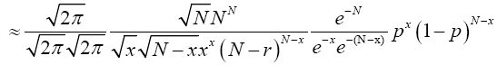
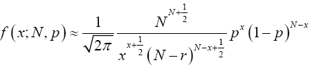
Multiplying both numerator and denominator by  , we have;
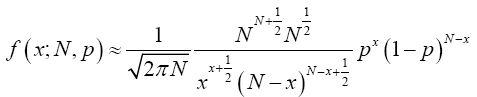
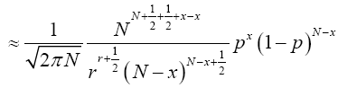
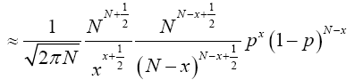
 (18)
(18)
Change variables x=Np+ε, ε measures the distance from the mean of the Binomial Np, and the measured quantity r. The
variance of a Binomial is Np(1-p), so the typical deviation of x from Np is given by 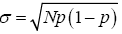 . Terms of the form
 will therefore be of order
 and will be small.
Re-write (18) in terms of ε.
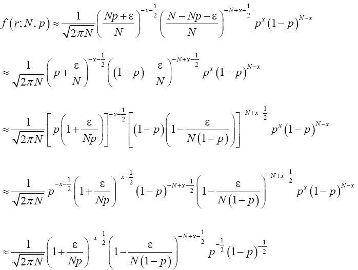
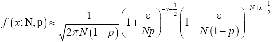 (19)
(19)
Rewrite (19) in exponential form to have
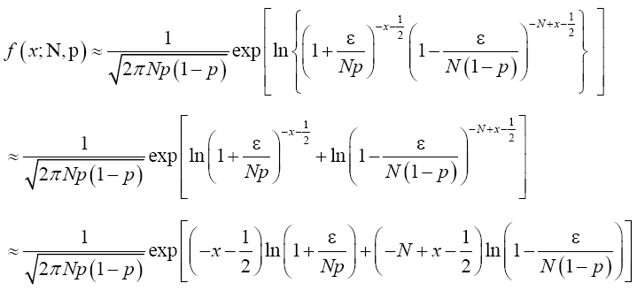
 (20)
(20)
Suppose f(x)=ln(1+x), using Maclaurin series 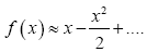 and similarly
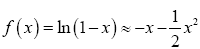 Therefore
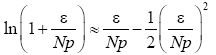 (21)
(21)
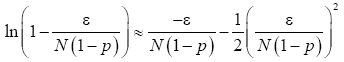 (22)
(22)
Putting (21) and (22) in (20) and simplify, we have
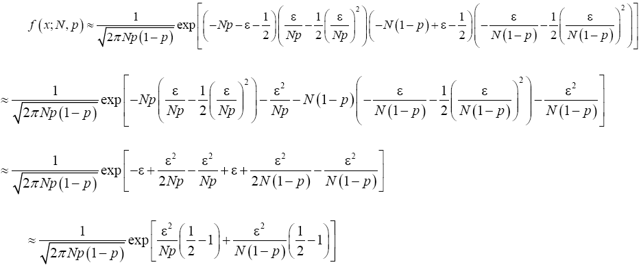
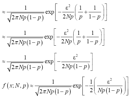
Recall that x=Np+ε which implies that ε2=(x-Np)2. From Binomial distribution Np=μ and Np(1-p)=σ2 which also implies that 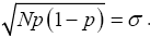 Making appropriate substitution of these in the equation (23) above provides;
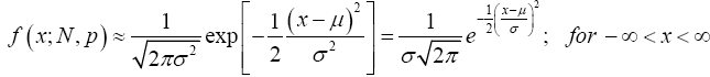 (24)
(24)
We have easily derived equation (24) that is popularly and generally known anywhere in the whole world as Normal or Gaussian distribution.
Definition 3.3 (Normal Distribution) A continuous random variable X has a normal distribution, is said to be normally distributed, and is called a normal random variable if its probability density function can be defined as follows: Let μ and σ be constants with -∞ < μ < ∞ and σ > 0. The function (24)
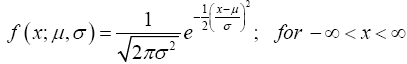
is called the normal probability density function with parameters μ and σ.
The normal probability density function is without question the most important and most widely used distribution in statistics [20]. It is also called the "Gaussian curve" named after the Mathematician Karl Friedrich Gauss.
To verify that equation (24) is a proper probability density function with parameters μ and σ2 is to show that the integral
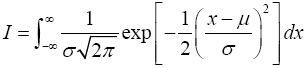
is equal to 1.
Change variables of integration by letting  which implies that dx=σdz. Then
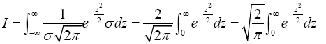
Now
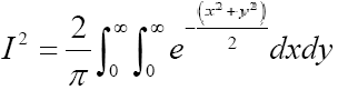
or equivalently
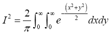
Here x; y are dummy variables. Switching to polar coordinate by making the substitutions x=r cos θ, y=r sin θ produces the Jacobian of the transformation as
 (25)
(25)
So
Put 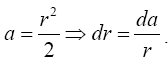 Therefore,
Thus I=1, indicating that (24) is a proper p.d.f.
It is now well-known that a Binomial r.v. is the sum of i.i.d. Bernoulli r.v.s, Poison r.v. arises from Binomial (n Bernoulli trial) with n increasing indefinitely, p reducing to 0 so that np=λ (a constant), Also, when n (number of trials in a Bernoulli experiment) increases without bound and p ≠ 0 and p ≠1 (that is, p is moderate), the resulting limiting distribution is Gaussian with mean (μ)=np and variance (σ2)=np(1-p). This our alternative technique provides a direct approach of convergence, this material should be of pedagogical interest and can serve as an excellent teaching reference in probability and statistics classes where only basic calculus and skills to deal with algebraic expressions are the only background requirements. The proofs are straightforward and require only an additional knowledge of Maclaurin series expansion, gamma function and basic limit concepts which were thoroughly dealt with in preliminaries section.