Keywords
|
| State vector, state transition function, covariance matrix, Jacobian matrix, filter gain |
INTRODUCTION
|
| The Kalman Filter represents one of the most widely applied and demonstrably useful tool, to emerge from the state variable approach of “Modern control theory”[1]. The Kalman filter is a prediction filter. Put in simple terms, the filter extracts the noise free measurements from a set of erroneous measurements, by estimating the state of the plant, whose parameters are measured. In doing so it tries to minimize the difference between the measurements and an estimate of the measurements. In fact, the original proposition by Gauss regarding the estimation by the method of least squares becomes the Kalman Filter, when the minimization problem, as given by Gauss, is given a recursive solution [Gauss to Kalman]. It is often observed that for linear systems, the deterministic theory based on mean square estimation and the probabilistic estimation theory are equivalent. |
THEORY OF KALMAN FILTER
|
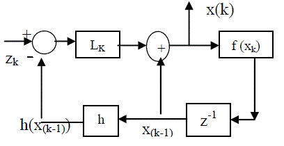
| As illustrated in Fig.1 consider a system represented by the dynamic equation |
| x(k+1) = f(x(k) + w(k) (1) |
| where f() is a nonlinear function that explains the state transition of the a system represented by the sate x(k) (w(k) is the plant noise, assumed to be Gaussian). A measurement device gets a set of measurements regarding the plant given |
| z(k) = h(x(k)) + V(k) ( 2) |
| where h () is a non linear function that transforms the state into the measurements. In other words, the measurements can be spelt out in terms of the state. V(k) is the measurement noise, which is also normally distributed. Given the measurement x(k) at time k, the filter updates the state x(k) in terms of the difference between the current measurement and an estimate of the measurement made on the basis of the past (k-1) estimates. |
| x(k) = x(k-1) + L(k)[ z(k) – h(x(k-1))] (3) |
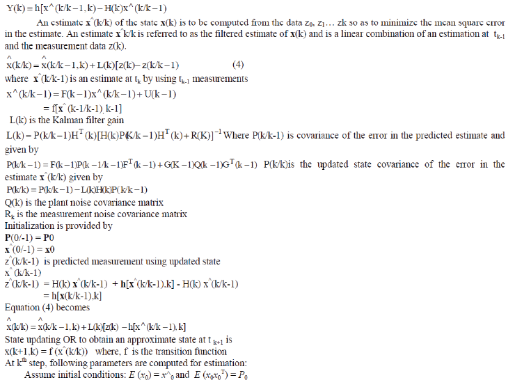
| L(k) is the Kalman gain, computed from the co-variance of the state vector and the Jacobean of the vector functions f and h. The updated state undergoes a temporal update using Eq. 1 generating x(k+1), which become the candidate for estimating the measurement at time k+1. As the filter converges, the variance of residual z(k) – h(x(k-1)) , remains bounded to specified limits. |
EXTENDED KALMAN FILTER
|
| A. Introduction |
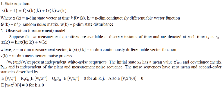
| Well-known method for estimation of state in linear systems with correlated noise is the extended Kalman filter, where the unknown parameters are estimated as a part of an enlarged state vector. In Extended Kalman Filter to estimate the state, by modelling the systems by state equations where the state consists of the system and noise parameters while the corresponding output, input and computed residuals are collected in the observation matrix of the state equations. The Kalman Filter requires an initial state for each object, and that initial state estimate must be obtained by detecting it. The system state vector xk is assumed to be describing a dynamic system having the form, |
 |
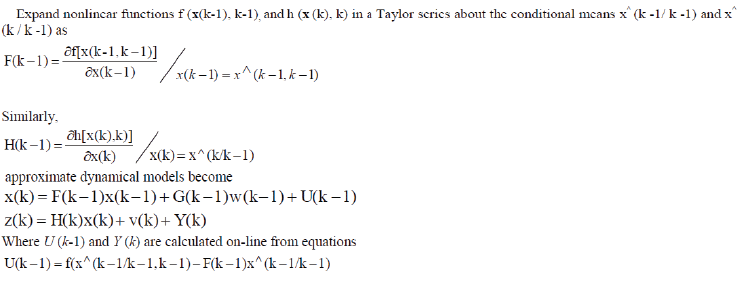
| where wk represents a white noise sequence vk represent the measurement errors that occur at each observation time. Suppose m measurement quantities are available at discrete instants of time and are denoted at each time tk as zk . Due to the measurement noise vk there is a difference between the observed value and estimated value and is called the residual. The residual associated with the kth measurement is rk = zk-h (x^k/k-1) where h (x(k/k-1)) is the estimate of the state by using previous measurement. The estimate is given as the linear combination of estimate predicted in the absent of new data and the residual rk. Thus, the mean square estimate is x^(k/k) = x^(k/k-1) + L (k) [ zk – h (x^k/k-1)] where L (k) is the Kalman filter gain. State updating or to obtain an approximate state at tk+1 is x(k+1,k)= f (x^(k/k)) where, f is the state transition function. Fig.1 illustrates the structure of Kalman filter. As the filter converges, the state sequence will represent the plant behaviour and the estimated measurement shall be free from noise. Also, the mean value of residual would to zero. |
B. Discrete kalman Filter Structure
|
| The Kalman filter provides an estimate of the state of the system at the current time based on all measurements of the system obtained up to and including the present time. |
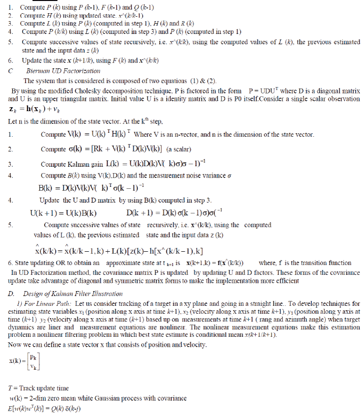
| The system that is considered is composed of two equations |
 |
 |
 |
 |
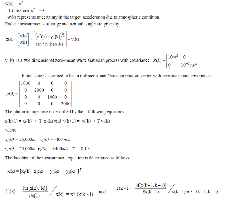 |
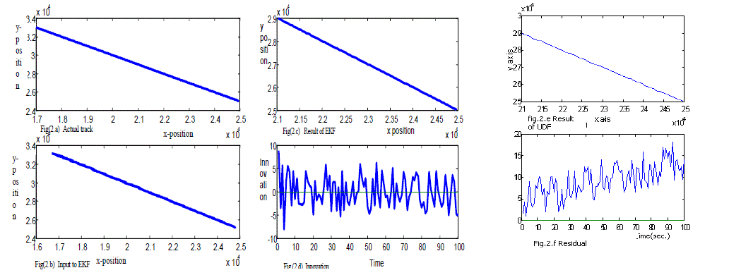
| Simulation of the extended Kalman filter for linear target tracking is shown in the accompanying Fig.(2). Fig. (2.a) shows the actual linear track of the object. Fig. (2.b) shows the track when the noise is added with the actual measurements.. Fig. (2.c) shows the output of the Kalman filter.. Fig (2.d) shows error (innovation) in the predicted states. Fig.(2.e) shows the output of the UD filter. UD factorization method generates the states correctly. Fig.(2.f) shows the residual variation in the estimated value. |
2) For non-Linear Path:
|
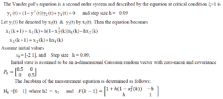 |
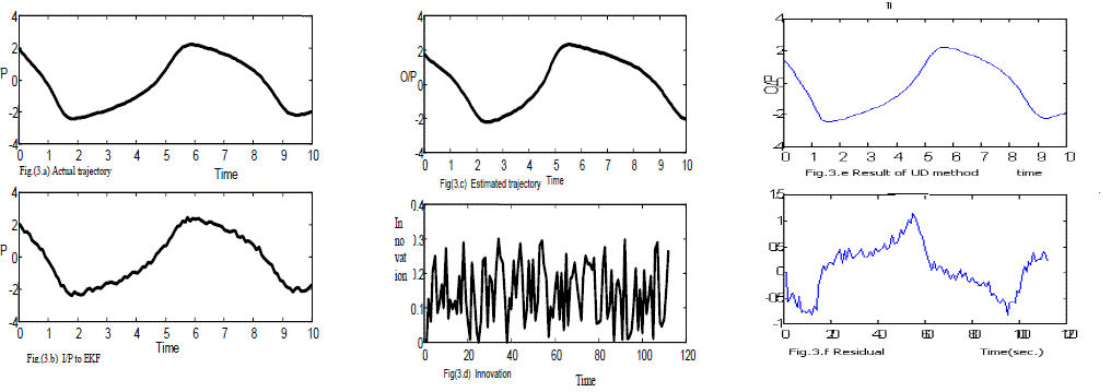
| Simulation result of the extended Kalman filter for this target trajectory are shown in the Fig.(3). Fig. (3.a) shows the actual trajectory of the object. Fig. (3.b) shows the track when the noise is added with the actual measurement data. This is the input of the Kalman filter. Fig.(3.c) shows the estimated trajectory. Fig.(3.d) shows the error(residual). Fig.(3.e) shows the output of the UD filter.. Fig.(3.f) shows the residual variation in the estimated value. |
CONCLUSION
|
| This work presents the practical aspects of implementing Kalman filter estimator applied to time varying stochastic non-linear models. The Kalman filter has found application in the tracking and navigation of all sorts of vehicles, and in predictive design of estimation and control systems. The UD Kalman filtering algorithm is considered efficient, stable and accurate for real time applications. In UD Factorization method, the covariance matrix P is updated by updating U and D factors. These forms of the covariance update take advantage of diagonal and symmetric matrix forms to make the implementation faster. This is one of the main advantages of the UD factorization method. |
ACKNOWLEDGMENT
|
| We take this opportunity to express our deepest gratitude and appreciation to all those who have helped us directly or indirectly towards the successful completion of this paper. |
Figures at a glance
|
 |
 |
 |
| Figure 1 |
Figure 2 |
Figure 3 |
|
References
|
- Kalman filtering: Theory and Practice, Mohinder S Grewal& Angus P Andrews, Prentice Hall
- Least Squares Estimation: From Gauss to Kalman, H.W.Sorenson (IEEE Sptrum, July 1970)
- Improved Extended Kalman Filter Design for Passive Tracking, H.Weiss& J.B. Moore, IEEE Transaction on Automatic Control, 1980
- Multi sensor data fusion, target tracking and classification, Presented to DEAL, Dehradun.1999 By Syama P Chaudhuri
- Sate estimation using an efficient square root filter during powered flight of a launch vehicle. S.K. Shrivastava, Conference on systems and signals 1986
- Kalman filtering with real time application. By C.K.Chui& G. Chen.
- Discrete square root filtering: A survey of current techniques, Paul G. Kaminski. IEEE Trans. Automat. 1971
- Decoupled Kalman filters for phased array radar tracking. Frederick E Daum IEEE Trans Automat. Mar. 1983.
|