International Journal of Advanced Research in Electrical, Electronics and Instrumentation Engineering
ISSN ONLINE(2278-8875) PRINT (2320-3765)
ISSN ONLINE(2278-8875) PRINT (2320-3765)
| Linash P. Kunjumuhammed Post doctoral fellow, Department of Electrical and Electronic Engineering, Imperial College London, United Kingdom |
| Related article at Pubmed, Scholar Google |
Visit for more related articles at International Journal of Advanced Research in Electrical, Electronics and Instrumentation Engineering
The paper illustrates a procedure to develop a dynamic simulation program for a single machine infinite bus (SMIB) test system using MATLAB/Simulink software. The program is useful to demonstrate various operational and stability challenges in power system operations. The method can be extended to make a program to simulate network having multiple synchronous machines, asynchronous machines, FACTS devices, dynamic load etc.
Keywords |
||||||||||||||||
| Power system dynamics, modelling, Synchronous machines, MATLAB, Simulink | ||||||||||||||||
INTRODUCTION |
||||||||||||||||
| Modelling and simulation studies are an integral part of power system analysis. They are used in the electricity related industry from the early days of digital computers. They are used to study the operation and stability of the system, controllers design and testing, operator training etc. | ||||||||||||||||
| This paper deals with programming of a single machine infinite bus (SMIB) test system using MATLAB/ Simulink software and intended for a complete beginner in the field of power system analysis. A basic methodology for developing a simulation program is discussed without detailing the theory behind the model. The program can be modified to include multiple synchronous machines, asynchronous machines, FACTS devices, dynamic load etc. | ||||||||||||||||
| The paper is divided into four sections. Following the introductory section, the Section II deals with the modelling aspects of a power system and lists key equations for dynamic model of a synchronous machine. The Section III explains the procedure for translating the dynamic model into a Simulink model. Results of an SMIB test system simulation are discussed in Part IV and several suggestions for possible future work are detailed. | ||||||||||||||||
DYNAMIC MODELLING OF POWER SYSTEM |
||||||||||||||||
| A model of a power system is an integration of several dynamic models such as synchronous generators, asynchronous generators, load, FACTS devices, etc. Fig. 1 shows a top level view of the model, where various dynamic models are connected to a network model. The output of the network model is fed back to the dynamic models making it a closed loop system. The network model consists of all transmission network components except the components modeled separately. It is represented using an algebraic equation V = Z I where V is a vector of bus voltage, I is a vector of injected current at each bus where the dynamic components are connected and Z is a matrix representing the impedance of transmission line and other components not modelled separately. (In some system studies, a more detailed model of transmission network using differential equations is used.) The output of the network block, bus voltage, is fed to the dynamic models. The dynamic models consist of differential and algebraic equations (DAE), and the outputs are injected current at corresponding buses. | ||||||||||||||||
| An SMIB simulation presented in this paper contains only a synchronous machine model block and a network model block. The modelling of synchronous generator is a subject matter of many text books and literatures [1-3]. Models of varying degree of complexity are reported. Choice of a model is made depending on the type of phenomena being studied and available computational resource. The DAE equations for a transient model of synchronous machine are explained here. Theory behind these equations is not explained as it is beyond scope of this paper. | ||||||||||||||||
| A. Synchronous machine model | ||||||||||||||||
| A synchronous generator generally has two inputs, a torque input from a turbine coupled to its rotor and an excitation current to field winding in its rotor. The excitation current produces magnetic poles in the rotor. When the mechanical torque from turbine forces the rotor to rotate, a rotating magnet field will be created in the air gap which cuts the stationary coils in the stator, and induces a voltage in the stator winding. Hence the mechanical torque supplied by a turbine is converted to electrical torque through the flux linkage and transmitted to grid as voltage and current. | ||||||||||||||||
| Fig. 2 shows an internal block diagram representation of a synchronous machine model. It consists of three blocks, namely torque-angle loop, rotor electrical block, and excitation system block. | ||||||||||||||||
| The torque angle loop represents turbine and generator mechanical system. Inputs to this block are mechanical and electrical torques, and outputs are rotating speed and rotor position. If mechanical torque and electrical torque are balanced, the rotor will rotate at a constant speed called synchronous speed. A change in either of the torques will cause the speed to change. Another output of the block is the rotor position. Consider any fixed point in the rotor. For an outside observer, the point will rotate in a circle and hence the rotor position will change from 0 to 360 degree. However, if the observer is rotating at the synchronous speed, the point will look stationary. Now the rotor position represents the relative angle between the observer and the point. When an imbalance occurs in the torques, the observer will notice a change in the speed and the rotor position. In the dynamic synchronous machine model, parameters are resolved into the rotating observers frame, generally called rotating reference frame using Parks's transformation [2]. This paper does not describe details of this transformation. Readers are advised to refer relevant literature to understand this concept. | ||||||||||||||||
| The rotor electrical block represents flux dynamics in the machine windings. The excitation system block compares terminal voltage magnitude with a reference voltage, and outputs field voltage. There are two inputs for the synchronous machine model. One of them is the mechanical torque which is assumed to be constant during the course of simulation. The second one is terminal bus voltage vt obtained from the network block. The output of the model is current it which is fed to the network block. | ||||||||||||||||
| DAE equations corresponding to the individual blocks are listed below. This paper does not cover details of these equation as it is beyond its scope. [1-2] provides detailed analysis of these equations. | ||||||||||||||||
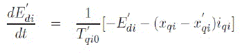
| 1) Equations for rotor electrical block | ||||||||||||||||
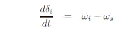 (1) (1) |
||||||||||||||||
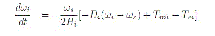 (2) (2) |
||||||||||||||||
 |
||||||||||||||||
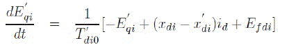
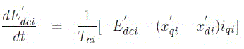
| 2) Equations for rotor electrical block | ||||||||||||||||
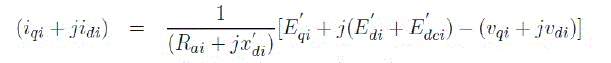
| One of the inputs to this block is the terminal voltage, Vt. It is a complex number which can be written as, Vt = vQi+jvDi. This voltage is transformed to a synchronously rotating reference frame as vqi+jvdi using (3). | ||||||||||||||||
 (4) (4) |
||||||||||||||||
 (5) (5) |
||||||||||||||||
 (6) (6) |
||||||||||||||||
| Equation (6) represents a dummy rotor coil used to handle transient saliency. A detailed discussion on treating saliency is available in [1]. | ||||||||||||||||
 (7) (7) |
||||||||||||||||
 |
||||||||||||||||
| 3) Excitation system block | ||||||||||||||||
| The block diagram representation of a static excitation system is shown in Fig. 3 [1]. Vt and EFD are input, the magnitude of terminal voltage and output, the field voltage, respectively. The regulator transfer function has a single time constant TA and positive gain KA. | ||||||||||||||||
DEVELOPMENT OF A SIMULINK MODEL |
||||||||||||||||
| This section explains steps involved in building a simulink model to simulate an SMIB test system. The model described in the previous section contains several differential equations. Hence to start with, section \ref{sec_sec1} describes how to program a simple first order differential equation using the Simulink. In section \ref{sec_sec2}, programming of the torque angle loop block is explained. | ||||||||||||||||
| A. Simulating a first order differential equation using Simulink | ||||||||||||||||
| Let us take a first order transfer function given by (10), | ||||||||||||||||
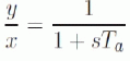 (10) (10) |
||||||||||||||||
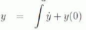
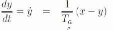 (12) (12) |
||||||||||||||||
 (13) (13) |
||||||||||||||||
| where y(0) is an initial value of the state y. The initial value indicates the value of a state under steady state, i.e. dy/dt=0. From (12), y(0) = x. | ||||||||||||||||
| Fig. 4 shows Simulink model for the transfer function in (10). The initial value y(0) is specified as a parameter in the integrator block. | ||||||||||||||||
| The power system model presented above consists of non-linear equations which call for a numerical solution. It is assumed that, the system is at a stable equilibrium point (SEP) at time t=0 and a disturbance happens at t>=0. To start the simulation, it is necessary to calculate the initial value of all machine states, x0 at time t=0. | ||||||||||||||||
| B. Calculating initial conditions for the SMIB model | ||||||||||||||||
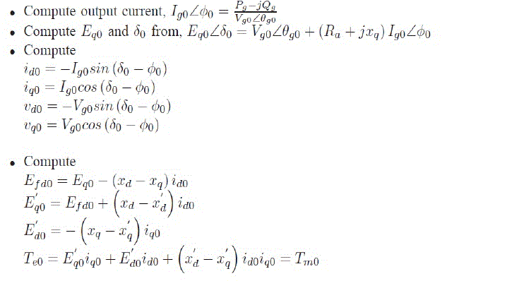
| The primary step in initializing the model is to obtain a power flow solution of the network. The power flow solution gives real and reactive power output of generators Pg and Qg, and terminal voltage magnitude and angle Vt and θt at buses. At SEP, the change in value of the states with time is zero which means, the d/dt term in all differential equations can be set to zero and the initial value of states can be deduced. A step by step procedure for initial value computation for the synchronous machine specific to this work is listed below. A more detailed explanation is available in [2]. The subscript 0 in the following equations indicates initial value or steady state value of the state variables. | ||||||||||||||||
 |
||||||||||||||||
| C. Simulating torque and loop block using Simulink | ||||||||||||||||
| The torque angle loop block contains two first order differential equations (1, 2). At steady state, both dδ/dt and dω/dt are equal to zero and the initial value of ω and Tm can be computed. Following the method described in Section III-A, a Simulink model for torque angle loop can be built as shown in Fig.5. | ||||||||||||||||
| Similarly, differential equations corresponding to rotor electrical blocks can be programmed as shown in Fig. 6. The static excitation system block is essentially a first order transfer function and is programmed similar to Fig. 4. | ||||||||||||||||
SIMULATION RESULTS |
||||||||||||||||
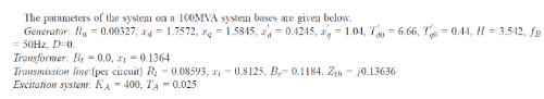
| An SMIB system shown in Fig. 7 is used to demonstrate the programming. In the test system a synchronous machine is connected to a grid through a transformer and a double circuit transmission line [2]. The grid is represented using impedance connected to an infinite bus. The infinite bus means that the bus has fixed voltage and frequency. The system can be used to study the interaction of the generator with the grid. | ||||||||||||||||
 |
||||||||||||||||
| A. Steady state operating condition of the SMIB test system | ||||||||||||||||
| Under steady state the active and reactive power output of the machine are assumed as Pt = 0.6, Qt = 0.0228. For an infinite bus voltage EB = 1.0, the terminal voltage of the generator is calculated as Vt = 1.05< 21.83. Using the method described in the Section III-B following initial values are computed. δ0= 61.5 degree, E'q0 = 0.9704, E'd0 = -0.2314, id0 = -0.3825, iq0 = 0.4251, Efd0 = 1.4802, Tm0 = 0.6011. | ||||||||||||||||
| B. Response of the SMIB system to step change in infinite bus voltage | ||||||||||||||||
| A step change in the infinite voltage is applied at time t=1 which is plotted in 8(a). The dynamic response of Vt, Pg, Qg, Te, δ are plotted in Fig. 8(b) to Fig. 8(f). The variation in δ following the disturbance is with respect to the rotating reference frame. | ||||||||||||||||
| C. Suggestions for further work | ||||||||||||||||
| The simulation set up described in this paper can be used to analyze the response of the machine under various system disturbances. Few examples are, three phase fault, transmission line trip, change in excitation reference voltage, change in input mechanical torque. A governor model can be added to the program to study the frequency response of the synchronous machine. | ||||||||||||||||
| A state space model of the system can be obtained using the linmod command and the eigenvalues can be computed using eig commands available in MATLAB. It is possible to explore possibility of designing a power system stabilizer for this system. | ||||||||||||||||
| The concept explained in this paper can be extended to make a multi-machine system simulation with asynchronous generators and FACTS devices. | ||||||||||||||||
CONCLUSION |
||||||||||||||||
| A programming approach for simulating a power system using MATLAB/ Simulink is discussed in this paper. The concept is explained using a SMIB test system simulation. The dynamic response of the test system to a disturbance in the grid is presented to further illustrate the method and several suggestions for further development are listed. | ||||||||||||||||
Figures at a glance |
||||||||||||||||
|
||||||||||||||||
References |
||||||||||||||||


