1Department of Statistics, Addis Ababa University, Addis Ababa, Ethiopia
2Johann Bernoulli Institute of Mathematics and Statistics, University of Groningen, Groningen, The Netherlands
Received date: 10/07/2016; Accepted date: 24/07/2016; Published date: 28/07/2016
Visit for more related articles at Research & Reviews: Journal of Statistics and Mathematical Sciences
Four major crop producing regions in Ethiopia, i.e., Tigray, Amhara, Oromia and SNNP were included in the study. Three models for production function: linear, exponential and Cobb Douglas were considered and assessed for statistical model diagnostics. The statistical model diagnostics suggested that crop production function was found to be represented by the Cobb-Douglas function based on data from 2007/2008 agricultural sample survey. The Cobb-Douglas production function was first fitted using ordinary least squares (OLS). As expected, the parameter estimates using OLS were misleading due to occurrence of outliers; hence robust regression was taken as an alternative. Then many of the parameter estimates received the expected signs, R2 values increased and standard errors of parameter estimates decreased. In general, farm size, fertilizer, seed, oxen power and human labor were important to maximize crop yield. The great contribution was found to be due to farm size in each of the regions except in SNNP where it was due to human labor. Education variable was found to be statistically insignificant and received negative sign in Tigray and Amhara. Production elasticities for each of the inputs except farm size in Tigray, Amhara and Oromia suggested that the relation between inputs and output was inelastic.
Production function, Robust regression, Outliers, Crop production, Ethiopia, Cobb-Douglas, OLS, Tigray, Amhara, Oromia, SNNP
Agriculture in Ethiopia is the leading activity of the nation and hence the country’s economy is predominantly agrarian. It has on average accounted for about 50% of the overall GDP, generates 90% of export earnings and supplies about 70% of the country’s raw material to the secondary activities [1]. The major food crops are produced in almost all regions of the country in spite of the variation in volume of production across the regions. To this end, main season [2] production of major crops by private peasant holdings accounted on average for over 90% of total output of major crops and 93% of cultivated area in any one year [1].
Ethiopia grows large varieties of crops, which include cereals (‘teff’, corn, wheat, barley, sorghum, millet, oats, etc.); pulses (horse beans, chick-peas, haricot beans, field peas, lentils, soybean, and vetch); oilseeds (linseed, fenugreek, ‘noug’, rapeseed, sunflower, castor bean, groundnuts, etc.); stimulants (coffee, tea, ‘chat’, tobacco, etc.); fibers (cotton, sisal, flax, etc.); fruits (banana, orange, grape, papaya, lemon, ‘menderin’, apple, pineapple, mango, avocado, etc.); vegetables (onion, tomato, carrot, cabbage, etc.); root and tuber (potato, ‘enset’, sweet-potatoes, beets, yams, etc.) and sugarcane. According to the 2007/08 (2000 EC) annual crop production forecast survey, which was conducted by Central Statistical Agency (CSA) of Ethiopia, a total area of about 11 million hectares were covered by grain crops, i.e., cereals, pulses and oil seeds, from which a total of about 164.51 million quintals of grains were expected to be produced, from private peasant holdings.
Ethiopia has great agricultural potential because of its vast areas of fertile land, diverse climate, generally adequate rainfall, and large labor pool. Despite this potential, however, agriculture in Ethiopia has remained underdeveloped because it is plagued by periodic drought; soil degradation (which is caused by overgrazing, deforestation and high population density) and a poor economic base (low productivity, low land management, weak infrastructure and low level of technology). The existing backward and traditional farm tools and very limited use of modern farm inputs together with dominating rain fed agriculture, (where the performance of the sector is highly dependent on the timely onset, duration, amount and distribution of rainfall) have contributed a lot for the existing subsistence / hand to mouth / farming system.
In a country with dominating agrarian economy like Ethiopia, due attentions, (including extensive research works) have to be given for increasing the performance of agriculture, in terms of total volume of production in order to secure domestic food availability for its population. To this verity, the government of Ethiopia has been devising and implementing various economy wide and sectoral policies and strategies. During the last one and half decade, the government has identified agriculture as a priority sector for development, and hence, devised the Agriculture Development Led Industrialization (ADLI) strategy. In order to realize the millennium development goals, agricultural extension services were expanded and supplies and applications of modern inputs increased leading to some improvements of aggregate production particularly of cereals, pulses, and oil seeds.
Ethiopia grows a large variety of crops in which grains are the most important field crops and being the chief element in the diet of most Ethiopians. The principal grain crops are teff, wheat, barley, which are primarily cool-weather crops; and corn, sorghum, and millet which are warm weather grain crops. Teff is the most preferred crop grown in the cooler highlands, while sorghum is the principal lowland crop because it thrives well in semi-arid environments due to its hardy and drought resistant properties.
Statement of the Problem
The sound performance of agriculture warrants the availability of food crops. The principal role that agriculture plays in Ethiopia’s political, economic and social stability makes measures of agricultural productions extremely sensitive. Agriculture in Ethiopia is characterized by its low productivity. The reason for this is the use of limited modern agricultural techniques and traditional practices as well as the declining soil fertility due to continuous cropping. Among traditional practices used to increase the crop productivity, the most widely used practice has been and still maintaining is soil fertility through long fallow periods and the use of dung and crop residue. These gradually become impossible due to the prevailing rapid and uncontrolled population growth, which led to the reduction of the fallow lands and fuel wood deficit in the country. The other practice to increase crop production was based on expanding cultivable cropland. However, this scheme has been in practice for a long time and as a result of high population growth in the country most of the highlands suitable for cropping have already been exhausted.
Therefore, the only realistic option to raise the living standards of the rural population, to ensure food security and poverty alleviation is to focus on methods of increasing productivity of land and other resources while conserving those which are overutilized.
Farmers in Ethiopia are faced with key decisions on how best to produce crops and how much to produce, given their limited resources. The problems of low crop production include unavailability of enough crop land, the use of traditional agricultural technology (such as inappropriate application of chemicals and fertilizer amount) and poor distribution of other agricultural inputs. In connection with this, a study conducted by Addis et.al. [3] revealed that the main crop production problems in some selected woredas of the central highlands of Ethiopia were the lack of land, shortage of family household labor, high price of inputs, lack of loans from formal and informal sources, poor access to markets, shortage of appropriate storage facilities, and lack of extension services.
In view of the above issues, it is extremely imperative to deal with optimal production of crops. In general, several studies in the literature have employed production function analyses for the sake of handling problems of optimal production. A production function relates a single output y to a series of factors of production x1, x2, …, xn. In particular, crop production function relates the amount of crop yield per household to factors of production such as area of crop land, labour force participation, amount of fertilizer employed, amount of seed applied and amount of water applied.
In agricultural production function analysis, the marginal product forthcoming from a decision to increase or decrease a factor level depends on the available quantities of the other factors; e.g., the additional product yielded by an additional unit of fertilizer applied depends greatly upon the quantities of land, labor etc., combined with it. That is, one expects production inputs to be technically interdependent; specifically, for normal inputs it is expected that an increase in an input level increases the marginal and average productivities of other inputs in the production process. In such cases, regression parameter estimation should address the problem of collinearity so that better trustworthy estimates of the parameters will be obtained.
Exceptionally low or high crop yields are ordinary in many crop production schemes. Additionally, there may happen to observe extreme values from among factors of crop production such as crop area, amount of fertilizer applied and number of plowing oxen in any farming system. The impact of exceptional values of such observations (outliers) is that the classical methods of obtaining estimates of parameters like least squares fitting criteria can produce misleading results. The problem of outliers has been treated by using robust regression techniques [4]. Thus, robust regression method is applied as a means of addressing the problem of outliers in this research so that the parameter estimates, which are obtained from a given production function, will no longer be misleading. Moreover, the adequate representation of production or crop yield functions is crucial for modeling purposes in agricultural and environmental economic analyses. To this end, the discussion and estimation of different functional forms of production function has gained much attention in agronomic and agricultural economics literatures.
Though there are few studies, which have been conducted on agricultural production and efficiency of farmers in some parts of Ethiopia [3-6], much attention has not been given to the estimation of crop production function in Ethiopia with the applications of statistical techniques such as robust regression. Therefore, this study attempts to show the application of robust regression on production function analyses for private peasant holdings crop farming system in Ethiopia, focusing on the most important factors of production affecting crop yield, such as crop area in hectares, labour, fertilizer, and seed.
Objectives of the Study
(i) To apply production function analysis for private peasant holdings crop farms in Ethiopia using robust regression.
(ii) To fit different crop production functions and choose the appropriate one for private peasant holdings crop farms based on data from the 2007/08 (2000 EC) agricultural sample survey in Ethiopia.
(iii) To analyze factors of crop production at different regions of private peasant holdings in Ethiopia.
Data an d method of analysis
The Data
The analysis and estimation of crop production function in this study employed data from the 2007/08 (2000 EC) agricultural sample survey [2] (‘Meher’ season) conducted by Central Statistical Agency of Ethiopia. The agricultural sample survey covered the entire rural parts of the country except the non-sedentary populations of three zones of Afar and six zones of Somali regions. However, this research considered only the four major crop producing regions namely: Tigray, Amhara, Oromia and SNNP.
The Variables in the Study
The dependent variable: total crop production, denoted by Y is defined as the total amount of crop yield in quintals per private peasant holding.
Independent variables: the following independent variables were hypothesized to influence the crop yield in each of the study regions either positively (+), negatively (-), or positively and/or negatively (+/-).
(i) X1: Amount of chemical fertilizer employed in kilogram (+).
(ii) X2: Weight of improved and/or non-improved seed in kilogram (+).
(iii) X3: Area of agricultural land in hectares (+).
(iv) X4: Human labour, which is calculated based on the household size of the farmer (+).
(v) X5: Oxen labour: it is defined as the total number of plowing oxen a household own (+).
(vi) X6: Education (highest grade) attained by the head of the household (+).
(vii) X7: A dummy variable scoring 1 for respondents having extension contact and 0 otherwise (+).
(viii) X8: A dummy variable scoring 1 for damaged crops and 0 otherwise (-).
(ix) X9: A dummy variable scoring 1 for irrigated crop field and 0 otherwise (+).
(x) X10: A dummy variable scoring 1 if the crop land ownership type is private and 0 if the crop land ownership type is Rent/ Leased (+/ -).
The Production Functions
A production function is a function that specifies the output of a firm, an industry, or an entire economy for all combinations of inputs. Given the set of all technically feasible combination of output and inputs, only the combinations encompassing a maximum output for a specified set of inputs would constitute the production function. Alternatively, a production function can be defined as the specification of the minimum input requirements needed to produce designated quantities of output, given available technology. It is usually presumed that unique production functions can be constructed for every production technology.
The relationship of output to inputs is non-monetary, that is, a production function relates physical inputs to physical outputs, and prices and costs are not considered. But, the production function is not a full model of the production process: it deliberately abstracts away from essential and inherent aspects of physical production processes, including error and waste. The primary purpose of production function is to address allocative efficiency in the use of factor inputs in production and the resulting distribution of income to those factors. Under certain assumptions, the production function can be used to derive a marginal product for each factor, which implies an ideal division of the income generated from output into an income due to each input factor of production.
An appropriate production function (model) should exhibit several technical characteristics generally believed true of production processes. On an a priori basis, agricultural production function can be hypothesized to exhibit three essential characteristics. First, like most production processes, inputs in an agricultural process will likely follow the law of diminishing marginal productivity, i.e., as successive units of a variable input are applied to a given quantity of other resources, the resultant increments to output (marginal product) will decline. Secondly, the marginal product forthcoming from a decision to increase or decrease a factor level depends on the available quantities of the other factors. Finally, if one of the requisites for production is absent, i.e., a zero input level, the process would yield no output.
The technical characteristics of a production function, which are stated above, may not be strictly valid for any functional form considered in a given study; because model specifications having desirable technical properties are sometimes accompanied by statistical problems or simply not supported by the data. As a result, other functional forms, though they do not satisfy the stated technical characteristics should be considered for further analysis in view of statistical and mathematical desirability. Relaxing one or more of the above characteristics and based on a review of traditional and popular literatures, Griffin, et al. [7] identified twenty functional forms including linear, quadratic, square root, translog and Cobb-Douglas. The models considered in the estimation of production function in this research work, are: linear, Cobb-Douglas and exponential.
A production function can be expressed in the implicit form as:
i = 1, 2, 3, …, n ……. (1)
where,
• Yi is the output;
• X1i, X2i,…, XKi, are K explanatory variables (inputs);
• εi is the ith error term;
• n is the number of observations (cases) included in the study;
• f(.) is a known function of explanatory variables.
The different inputs for crop production function can be labor, land, seed, fertilizer, chemicals, and tractor (plowing oxen).
The Linear Production Function
 (2)
(2)
where,
• Y is the output or response (dependent) variable; X1
• X1, ... , XK are the K factors of production (inputs);
• n = the number of cases considered in the estimation of production function;
• i = 1, 2, 3, …, n
• βj′s are the parameters to be estimated.
• εi = The random disturbance term and is distributed independent-normal with mean zero and constant variance σ2.
The Cobb-Douglas Production Function
The Cobb-Douglas functional form given hereunder is frequently used in the literature and proved to accurately capture the underlying relationship [8,9].
Model: 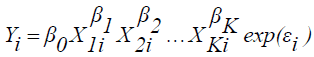 (3)
(3)
where, X1, ... , XK, Y, i and å are as defined above.
The model can be changed into linear form as follows so that the parameters will be estimated using the method of estimation for linear regression.
 (4)
(4)
The Exponential Production Function
 (5)
(5)
where, X1, ... , XK, Y, i and å are as defined above.
This model can also be transformed into linear form so that the parameters will be estimated using the method of estimation for linear regression.
 (6)
(6)
The Multiple Linear Regression Model and Statistical Assumptions
The empirical investigation of problems that result from a given data set should begin only after the model has been satisfactorily specified and further checked for statistical assumptions. Consider the following multiple linear regression models:
Y = Xβ+ε (7)
where,
• Y is an n x 1 vector of dependent variable;
• n is the number of cases/ subjects considered in the regression;
• X is an n x (K+1) matrix of independent variables;
• K is the number of explanatory variables;
• β is a (K+1) x 1 vector of regression coefficients and
• ε is an n x 1 vector of random disturbances.
Upon considering the above regression model, the following assumptions should be satisfied by the data set at hand, detail discussion can be found in Gujarati [10] among others.
(i) Linearity - the relationship between the predictors and the outcome variable should be linear.
(ii) Normality - the errors should be normally distributed. Technically normality is necessary only for the t-tests to be valid, but estimation of the coefficients only requires that the errors be identically and independently distributed.
(iii) Homogeneity of variance (homoscedasticity) - the error variance should be constant. Often the existence of a few extreme or unusual observations (outliers) in a homoscedastic model makes the model heteroscedastic [11]. The plot of residuals versus predicted values are important to see whether the assumption of homoscedasticity is violated or not. If the residuals have some patterns as a function of predicted values, then there will be an evidence of non-constant variance (heteroscedasticity). When the plot of residuals appears to deviate substantially from normal, more formal tests for heteroscedasticity should be performed [12] (Jason and Waters, 2002). Possible tests for this are the Goldfeld-Quandt test, the Breusch-Pagan test and the White test. However, Rana, et.al [11] confirmed that the above tests suffer a huge setback in detecting heteroscedasticity when outliers are present. Accordingly, they proposed a modified Goldfeld-Quandt (MGQ) test with the computational steps given hereunder.
(a) Likewise the classical Goldfeld-Quandt test, order or rank the observations according to the value of X that supposed to cause heteroscedasticity, beginning with the lowest X value.
(b) Omit central c observations, where c is specified a priori and then divide the remaining (n-c) observations into two groups each of (n-c)/2 observations.
(c) Check for the outliers by any robust regression technique, preferably use the robust Least Trimmed of Squares, LTS (see the detail on LTS at the end of this chapter) to fit the regression line. Then compute the deleted residuals for the entire data set based on a fit without the points identified as outliers by the LTS fit.
(d) For both the groups compute the Median of the Squared Deletion Residuals (MSDR) and compute the ratio MGQ = MSDR2/ MSDR1
Where,
• MSDR2 and MSDR1 are the medians of the squared deletion residuals for the smaller and the larger groups respectively. Under normality, the MGQ statistic follows an F distribution with numerator and denominator degrees of freedom each of (n-c-2(K+1))/2.
• K is the number of explanatory variables in the model.
(iv) Independence - the error associated with one observation is not correlated with the errors of any other observations (no autocorrelation). Autocorrelation is more common in time series data where the error terms of one or more consecutive periods are correlated. With cross sectional data, however, random sampling guarantees that different error terms are mutually independent, and autocorrelation is not an issue [13].
(v) The x’s are linearly independent (no multicollinearity) and hence rank (XT X) = rank (X) = K, which implies that (XT X)-1 exists. Multicollinearity is neither a specification error that may be uncovered by exploring regression residuals nor a modeling error but is a condition of deficient data [14]. The various techniques that are useful for detecting multicollinearity are the following.
Examination of correlation matrix: A very simple measure of multicollinearity is inspection of the off-diagonal elements of
the correlation coefficient,  If regressors Xiand Xj are nearly linearly dependent, then
  will be near unity.
Variance Inflation Factor (VIF): VIF =  where
where  is the squared multiple correlation coefficient between
  and
other explanatory variables. As tends toward 1 indicating the presence of a linear relationship in the x’s, the VIF for the
estimated coefficient of Xi tends to infinity. It is suggested that a VIF in excess of 10 is an indication that multicollinearity may be
causing problems in estimation [14].
and
other explanatory variables. As tends toward 1 indicating the presence of a linear relationship in the x’s, the VIF for the
estimated coefficient of Xi tends to infinity. It is suggested that a VIF in excess of 10 is an indication that multicollinearity may be
causing problems in estimation [14].
Eigenvalues and Condition Number (CN): If there are one or more near-linear dependences in the data, then one or more eigenvalues of XT X, say λ1,λ2 ,...,.λk will be small. The CN is supposed to measure the sensitivity of the regression estimates to small changes in the data and is defined as the ratio of the largest to smallest eigenvalue of the matrix (XT X) of the explanatory variables, i.e.,
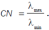 Generally, if the condition number is less than 100, there is no serious problem with multicollinearity. CN between
100 and 1000 imply moderate to strong multicollinearity, and if it exceeds 1000, severe multicollinearity is indicated.
Generally, if the condition number is less than 100, there is no serious problem with multicollinearity. CN between
100 and 1000 imply moderate to strong multicollinearity, and if it exceeds 1000, severe multicollinearity is indicated.
In addition to the above assumptions, there are issues that can arise during the analysis that, while strictly speaking, are not assumptions of regression, are none the less, of great concern to regression analysts. These are unusual observations, which may be outliers or leverage points that exert undue influence on the coefficients. The issue of satisfying the above assumptions and detecting outlying cases are intertwined. For example, if a case has a value on the dependent variable that is an outlier, it will affect the skew and hence the normality of the distribution. Detail discussion on outliers is given in the next section.
Whenever the above assumptions are entirely satisfied, the best (minimum variance) and unbiased linear estimator of in
equation 7 is obtained by the method of ordinary least squares (OLS). The method of OLS is based on minimizing the error sum
of squares 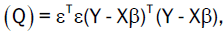 where T stands for transpose.
i.e,  (8)
(8)
Minimization of Q can be achieved by taking the partial derivative of Q with respect to each βi and equating to zero, i.e, 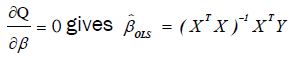 (9)
(9)
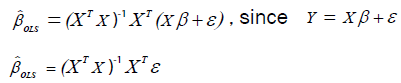
The above implies that 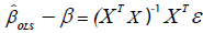
The expectation of 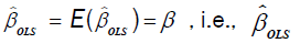 is unbiased since
The variance-covariance matrix of  is given by:
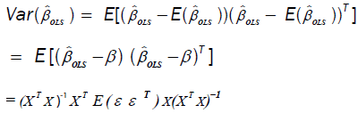
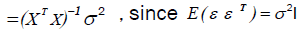 (10)
(10)
where σ2 is estimated by the mean square error, which is given by:
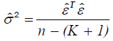 (11)
(11)
where, 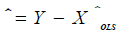 and n, K, T and
  are as defined above.
However, we are expecting that the crop production data in this research are vulnerable to unusual observations in such a way that the parameter estimates of OLS regression are misleading. As a result, a special attention is given to deal with regression analysis in the presence of unusual observations.
Unusual Observations and Robust Regression
Outliers: Outliers are observations that are numerically distant from the rest of the data. An observation with an extreme value on a predictor variable is a point with high leverage. Leverage is a measure of how far an independent variable deviates from its mean. If such leverage point deviates from the linear relationship described by the majority of observations it is called ‘bad leverage point’. In contrast, a leverage point is called ‘good leverage point’ if it does not deviate from the typical relationship. Good leverage points are not outliers and even improve the regression inference as these points reduce standard errors of coefficient estimates. Outliers can occur by chance in any distribution, but they are often indicative either of measurement error or that the population has a heavy tailed distribution.
A frequent cause of outliers is a mixture of two distributions, which may be two distinct sub-populations, or may indicate "correct trial" versus "measurement error" this is modeled by a mixture model. Outliers, being the most extreme observations, will include the sample maximum or sample minimum or both, depending on whether they are extremely high or low. However, the sample maximum and minimum need not be outliers, unless they are unusually far from other observations. Moreover, exceptionally low or high crop yields as well as extreme input values are ordinary in many crop production schemes. We particularly expect that production inputs are influential. For instance, the level of education can influence the appropriate use of modern agricultural practices and thus indirectly increases yield level. The response to plowing oxen and human labor can also change under greater and smaller number of cases. The impact of exceptional observation values (outliers) is that the least squares estimation is inefficient and can be biased.
Automatic rejection of outliers is not always a very wise procedure. Sometimes the outlier is providing information which other data points cannot due to the fact that it arises from an unusual combination of circumstances which may be of vital interest and requires further investigation rather than rejection. As a general rule, outliers should be rejected out of hand only if they can be traced to causes such as errors in recording the observations or in setting up apparatus [15]. The problem of outliers has been treated by using robust regression techniques [4]. Thus, robust regression method is applied as a means of addressing the problem of outliers/ leverage points in this research so that the parameter estimates will no longer be vulnerable as least squares estimates to unusual data.
Robust regression
A statistical procedure is regarded as robust if it performs reasonably well even when the assumptions of the statistical model are not true. Robust regression procedure generally refers to one that not only performs well if the population of errors is normally distributed but also is insensitive to small departures from the normality assumption. In the estimation of statistical regression models and testing the assumptions, one frequently finds that the assumptions are substantially violated. Sometimes the variables can be transformed as a means to conform the assumptions. Often, however, a transformation will not eliminate or attenuate the leverage of influential outliers that bias the prediction and distort the significance of parameter estimates. In such cases, robust regression that is resistant to the influence of outliers may be the only reasonable recourse.
Outlier detection
Outlier detection, one purpose of robust regression involves the determination whether the residual is an extreme negative or positive value. In the case of simple linear regression analysis, outliers can be detected using the scatter plot. However, this becomes impossible if the dimension of the problem exceeds the simple linear regression case and the number of observations is very large. Making use of residual plots as outlier diagnostic is a bad practice since residual plots might suffer from outliers [4], especially in the case of bad leverage points, i.e., outliers can tilt the regression line and have small regression residuals. As a result, other diagnostic tools are required to identify outlying or influential observations. In practical considerations, one often tries to detect outliers using diagnostics from a least squares procedure. Such procedures, however, are susceptible to the so called masking effect since they can be affected by extreme observations so strongly that the fitted model will fail to detect observations, which deviate from others. Outlier diagnostic procedures such as Student zed and jackknifed residuals, Cooks distances and Hat matrix elements also suffer from masking effect. Above all, in cases when two or more outliers are present, these outlier diagnostics may be able to detect only one since one outlier can be masked by other(s). To avoid this effect, robust methods of outlier detection have been employed in the literature.
Types of Robust Regression
There are many types of robust regression methods. Although they work in different ways, they all give less weight to observations that would otherwise influence the regression line. The main purpose of robust regression is to detect outliers and provide resistant (stable) results in the presence of outliers. Three classes of problems have been addressed with robust regression techniques:
(i) Problems with outliers in the y-direction (response direction)
(ii) Problems with multivariate outliers in the x-space (i.e., outliers in the covariate space, which are also referred to as leverage points)
(iii) Problems with outliers in both the y-direction and the x-space.
Methods of robust regression in response to the above problems include: least absolute values regression or least absolute deviation (LAD) regression, M-Estimation (Huber estimators and Bisquare estimators) and Bounded Influence Regression (least median of squares and least-trimmed squares).
High breakdown point: The robustness of an estimate against heavier data contamination is measured by its breakdown point, which is the largest proportion of outliers that can occur in a sample without entailing the possibility of arbitrarily large bias. Since one unusual observation (outlier) is enough to influence the coefficient estimates of OLS regression, the breakdown point for OLS regression is 0%. The maximum possible breakdown point is 50%. This is achieved by the least-trimmed-squares (LTS) estimate and least median of squares estimate, which is the estimate that minimizes the median of the squared residuals.
Least absolute deviation (LAD) regression: LAD regression unlike least squares regression minimizes the sum of the absolute values of residuals in order to estimate the regression coefficients. The strength of LAD estimation is that its robustness to the distribution of the response variable (although not with respect to the explanatory variable). For this reason, LAD estimates are sometimes recommended as starting values for iterative estimation algorithms. LAD method is especially suitable when the distribution produces a larger proportion of outliers than normal or when the sample is very large. Though LAD regression is robust to outliers, it is typically worse than OLS for cases with high leverage. If a leverage point is very far away, the LAD regression line will pass through it i.e., its breakdown point is also 0%.
M-estimates: The main advantage of LAD estimates over OLS is that they are not so sensitive to outliers. When there are no outliers, however, OLS estimates may be more accurate. M-estimates combine the advantages of both methods. In the case of high leverage, the performance of M-estimates falls down, meaning that the breakdown point is also 0%. M-estimation is a commonly used method for outlier detection and robust regression when contamination is mainly in the response direction.
Bounded influence (BI) methods: Despite M estimates are more efficient than LAD estimates; a single leverage point can completely dominate the ensuing estimate. This limitation has led to the development of estimates that bound the influence of any single element or row of X so that they guard against leverage points as well as regression outliers. Furthermore, these methods, which comprise least-trimmed-squares (LTS) estimates and least median of squares estimates have a much higher breakdown point as high as 50%. However, the efficiency of BI methods is less when the sample size under consideration is small.
Least-Trimmed Squares (LTS): LTS regression is based on the subset of h observations (out of a total of n observations) whose least squares fit possesses the smallest sum of squared residuals. The method of LTS regression is performed as follows.
Order the squared robust residuals from smallest to largest, i.e., 
Calculate  the LTS estimates of the regression coefficients by minimizing the sum of the squared robust residuals:
  where h is defined in the range:
  and by default SAS takes h as
  (SAS Institute [16],
2008) and K is the number of independent variables.
(SAS Institute [16],
2008) and K is the number of independent variables.
Above all, iteratively reweighted least square regression is applied for the estimation of production function (models) considered in this study, using the robustreg procedure of SAS9.2.
The data contamination in the crop production function is mainly in the response direction and hence the following M-estimation method can be employed. In M-estimation, the goal is to choose the regression coefficients that minimize some function of the residuals. The method of ordinary least squares has as its solution the coefficients that minimize the sum of squared residuals. This solution is undesirable when the data contain outliers, since an observation with a large error term will have a much larger effect (relative to the other observations) on the estimated coefficients.
Consider the linear regression model: 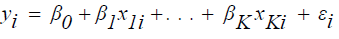 (12)
(12)
The most commonly used M-estimates, the Huber M-estimates,  are the values of
  that
minimizing the function :
that
minimizing the function :
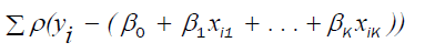 (16)
(16)
Where 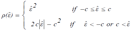 (14)
(14)
It is suggested to take c = 1.5σˆ , where σˆ is an estimate of the standard deviation σˆ of the population of random errors.
In order to find the minimum of (3.15), for a fixed value of σˆ , take the derivative of (3.15) with respect to and set each of them equal to zero. This yields K + 1 equations in K + 1 unknowns:
 (15)
(15)
for j = 0, 1, …., K, where one lets Xio=1 for all i. These are non-linear equations in the unknowns but they can
be approximated by linear equations as follows.
Consider an iterative procedure in which  are current estimates and
  represent improved
estimates.
represent improved
estimates.
Let 
In order to solve for the improved estimates, write 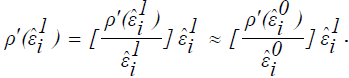
Let further that 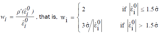
Then 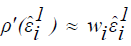 and one can estimate equation (15) by the linear equations:
 (16)
(16)
Let W be the diagonal matrix with diagonal entries  Then equation (15) can further be expressed in terms of matrix as:
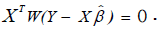
where,
(i)  is a K+1 by 1 vector of estimated regression coefficients;
(ii) X is an n by K + 1 design matrix;
(iii) Y is an n by 1 vector of response variable.
Solving the above equation for , one can obtain the following weighted least squares estimator.
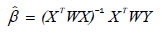 (17)
(17)
The iterative reweighted least squares can be started by setting  the vector of least squares estimates. At each iterative
step, the vector of current estimates is used to calculate the vector
the vector of least squares estimates. At each iterative
step, the vector of current estimates is used to calculate the vector 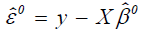 of residuals. Then use residuals to obtain
  and weights Wi. The vector of improved estimates can now be computed as in equation (17). The iterative procedure
continues until convergence.
and weights Wi. The vector of improved estimates can now be computed as in equation (17). The iterative procedure
continues until convergence.
In cases when data are contaminated in the x-space (this is what we normally anticipate in this research), M estimation does not do well [16] . As a result, the coefficient estimates of the iterative reweighted least squares regressions are obtained from the method of least trimmed squares (LTS). Since the efficiency of LTS estimation is low, the estimates obtained from this method can no longer be reliable and hence LTS estimation is only used as a means of outlier detection. Consequently, the final estimates of parameters are obtained from the weighted least squares fit in which weights can be determined as follows.c
Upon employing the method of iteratively reweighted least squares using LTS estimation, the diagonal elements of the
weighting matrix 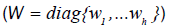 are generated by an indicator function,
 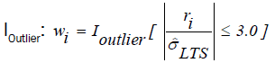 (18)
(18)
where,
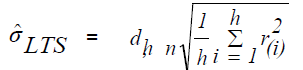
 is the scale estimate which can be obtained as follows.
 and
and  is chosen to make
  consistent assuming a Gaussian model.
Specifically, 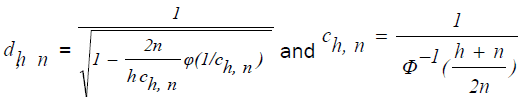
With Φ and ϕ being the distribution function and the density function of standard normal distribution, respectively.
ri is the residual obtained from LTS estimation.
(a) The above indicator function generates weights of zero for observations that are identified as outliers and weights of one otherwise.
(b) The cutoff value 3 is chosen from the fact that if the residuals are normally distributed, then roughly 99% of the standardized residuals will lie in the interval [-3.0, 3.0]
Finally, the coefficient estimates for weighted least squares are obtained with the help of equation (17) and these estimates are considered further for the interpretation of the final model.
Description of the Study Variables
The average amounts of crop production by private peasant holdings of Tigray, Amhara, Oromia and SNNP regions in the surveyed year were 17.36; 22.02; 32.89 and 30.74 quintals respectively with respective mean agricultural land areas of 1.24; 1.49; 2.22 and 1.25 hectares used for production. Despite the mean crop land owned by private peasant holdings in SNNP region was less than Amhara region and nearly the same as Tigray region, the above results show that the average crop production (yield) per peasant was the highest in SNNP region from among the three. This further indicates that average productivity was higher in SNNP region compared to Amhara region with a given mean area of crop land. The above results also imply that farmers in each region owned very small areas of agricultural land in which the mean area was less than 1.50 hectares at each of the regions except Oromia and this probably brought about the small mean crop yield per peasant in general. Table 1 also shows that the coefficients of variation (CVs%) for crop yield in Tigray, Amhara, Oromai and SNNP regions were 64.86; 65.85; 57.09 and 77.62 respectively so that the yield data were highly variable in SNNP region while they were the most stable in Oromia region. The maximum amount of crop yield in quintals was recorded at SNNP region whereas the minimum was at region Tigray (Table 1). Although the minimum area of agricultural land in hectare was almost the same at each region, the maximum being at Oromia region was exceedingly the highest as it is revealed in Table 1.
| Region | Variable | Number of cases | Minimum | Maximum | Mean | Median | Std. Deviation | CV% |
|---|---|---|---|---|---|---|---|---|
| Tigray | Education | 1676 | 0 | 12 | 2.29 | 1.00 | 2.28 | 99.56 |
| Family size | 1676 | 1 | 11 | 3.4 | 3.00 | 1.87 | 55 | |
| Fertilizer | 1676 | 0.00 | 335 | 45.04 | 30.44 | 41.31 | 91.76 | |
| Weight of seed | 1676 | 2.50 | 425 | 88.07 | 69.79 | 71.67 | 81.38 | |
| Area of land | 1676 | 0.03 | 6 | 1.24 | 1.02 | 0.86 | 69.35 | |
| Production | 1676 | 0.17 | 34.75 | 17.36 | 9.79 | 11.26 | 64.86 | |
| Number of oxen | 1676 | 0 | 6 | 1.74 | 2.00 | 0.75 | 43.1 | |
| Education | 6157 | 0 | 12 | 1.81 | 1.00 | 1.93 | 106.63 | |
| Family size | 6157 | 1 | 12 | 5.21 | 5.00 | 2.05 | 39.35 | |
| Amhara | Fertilizer | 6157 | 0.00 | 710 | 56.19 | 40.00 | 99.52 | 177.11 |
| Weight of seed | 6157 | 3.00 | 625 | 110.3 | 72.84 | 121.98 | 110.59 | |
| Area of land | 6157 | 0.26 | 8.25 | 1.49 | 1.26 | 1.08 | 72.48 | |
| Production | 6157 | 1.007 | 45.5 | 22.02 | 14.06 | 14.39 | 65.35 | |
| Number of oxen | 6157 | 0 | 9 | 1.5 | 1.00 | 0.87 | 58 | |
| Education | 6371 | 0 | 12 | 2.87 | 1.00 | 3.17 | 110.45 | |
| Family size | 6371 | 1 | 13 | 6.04 | 6.00 | 2.4 | 39.74 | |
| Oromia | Fertilizer | 6371 | 0.001 | 550 | 125.8 | 90.00 | 115.72 | 91.99 |
| Weight of seed | 6371 | 1.00 | 600 | 164.6 | 133.00 | 127.18 | 72.27 | |
| Area of land | 6371 | 0.05 | 11.67 | 2.22 | 1.89 | 1.52 | 68.47 | |
| Production | 6371 | 1.14 | 60.5 | 32.89 | 17.71 | 18.78 | 57.09 | |
| Number of oxen | 6371 | 1 | 12 | 2.03 | 2.00 | 1.09 | 53.69 | |
| Education | 8084 | 0 | 12 | 2.76 | 1.00 | 3.07 | 111.23 | |
| Family size | 8084 | 1 | 14 | 4.79 | 4.00 | 2.33 | 48.64 | |
| SNNP | Fertilizer | 8084 | 0.00 | 658 | 27.04 | 15.65 | 45.98 | 170.04 |
| Weight of seed | 8084 | 1.00 | 681.6 | 45.14 | 25.00 | 60.11 | 133.16 | |
| Area of land | 8084 | 0.05 | 10.35 | 1.25 | 0.93 | 1.56 | 124.8 | |
| Production | 8084 | 0.86 | 66.43 | 30.74 | 16.34 | 23.86 | 77.62 | |
| Number of oxen | 8084 | 0 | 14 | 0.85 | 2.00 | 1.42 | 167.06 |
Table 1: Summary statistics for continuous predictors and the dependent variable of crop production function in each region.
Peasants at each region completed an average of less than 3 years of schooling; the highest being 12 complete in all cases (Table 1). This indicates that farmers were relatively of low educational status with mean level attaining below second cycle primary education (grades 5 - 8). Table 1 also reveals that the mean value of weight of seed employed in Kg was the highest at Oromia region (164.64 Kg) but the lowest was observed at SNNP region (45.14 Kg). Yet the data on weight of seed employed in Kg were highly stable at Oromia region from among the entire regions since the CV% for weight of seed employed in Kg at Oromia region was the minimum (72.27). This implies that farmers in Oromia region applied relatively uniform amounts of seed as compared to farmers in the remaining regions. On the other hand, the data on weight of seed employed in Kg were highly variable at SNNP region, which further indicates that some peasants in the region applied high amounts of seed while others applied relatively small (Table 1).
In terms of the mean amounts of fertilizer employed in Kg that are given in Table 1, Oromia region took the highest (125.79 Kg) compared to the remaining regions. On the other hand, the lowest mean amount of fertilizer employed in Kg was corresponding to SNNP region (27.04 Kg). This by and large indicates that farmers applied small amounts of fertilizer in their crop production process. Furthermore, the values of coefficients of variation given at Table 1 reveal that the amounts of fertilizer used in Kg were greatly variable within peasants at Amhara region (CV% = 177.11) in which some of the peasants used high amount while others used small or not at all. Whereas, the data on amounts of fertilizer applied in Kg were relatively stable at Tigray region (CV% = 91.76), indicating that farmers in Tigray region used relatively similar amounts of fertilizer than farmers in the other regions.
Although the median number of individuals per household was greatest at Oromia region (6 persons), the maximum number of individuals in a household was observed at SNNP region (14 persons). Additionally, the values of coefficients of variation for number of individuals in a household show that, the data were relatively stable at Amhara region (CV% = 39.35), which indicates comparatively uniform family size per household. The maximum number of plowing oxen owned by a peasant was observed at SNNP region (14 plowing oxen) followed sequentially by Oromia (12), Amhara (9) and Tigray (6). The median number of plowing oxen owned by a peasant as indicated in Table 1 was small at each region in which it did not exceed two in any of the regions. This shows that number of plowing oxen, which is generally believed as being one of the most important inputs of crop farming in Ethiopia, was not fairly adequate. Moreover, the data on number of plowing oxen were greatly variable with coefficient of variation 167.06% at SNNP region, which reveals that some of the peasants owned greater number of plowing oxen while others possessed few or zero (Table 1).
Generally speaking, more than half of the peasants in each of the regions except Amhara (only 45.3%) had extension contacts (Table 2). Inspection of Table 2 also shows that the proportion of peasants, who applied irrigation, was generally low in each of the regions from which the highest proportion being observed at Tigray region (42.8%). Although Ethiopia has a good potential for developing irrigation, the above results indicate that irrigation was not highly practiced by peasants in each region. Perhaps, this is partly because irrigation requires a long-term effort and substantial investment, which is unlikely to implement it at the private peasant level owing to shortage of technical and financial resources. The descriptive results given above also reveal that the proportions of private agricultural land ownership by farmers in each region were high as compared to rented and/ or leased agricultural land. Though the mean size of crop land was generally small, the results in Table 2 reveal that most of the peasants owned agricultural land. In addition, the results in Table 2 show that crop damage was generally high in each of the regions. This probably led to minimum crop yield per peasant at each of the regions.
| Region | |||||||||
|---|---|---|---|---|---|---|---|---|---|
| Tigray | Amhara | Oromia | SNNP | ||||||
| Variable | N | Percent | N | Percent | N | Percent | N | Percent | |
| Extension | Yes | 862 | 51.4 | 2792 | 45.3 | 4068 | 63.9 | 5050 | 62.5 |
| Contact | No | 814 | 48.6 | 3365 | 54.7 | 2303 | 36.1 | 3034 | 37.5 |
| Total | 1676 | 100 | 6157 | 100 | 6371 | 100 | 8084 | 100 | |
| Irrigation | Yes | 717 | 42.8 | 2498 | 40.6 | 2392 | 37.5 | 3415 | 42.2 |
| Applied | No | 959 | 57.2 | 3659 | 59.4 | 3979 | 62.5 | 4669 | 57.8 |
| Total | 1676 | 100 | 6157 | 100 | 6371 | 100 | 8084 | 100 | |
| Crop damage | Yes | 1107 | 66.1 | 3721 | 60.4 | 3950 | 62 | 5152 | 63.7 |
| No | 569 | 33.9 | 2436 | 39.6 | 2421 | 38 | 2932 | 36.3 | |
| Total | 1676 | 100 | 6157 | 100 | 6371 | 100 | 8084 | 100 | |
| Land | Private | 1167 | 69.6 | 4541 | 73.8 | 4552 | 71.4 | 5556 | 68.7 |
| Ownership type | Rent/ Leased | 509 | 30.4 | 1616 | 26.2 | 1819 | 28.6 | 2528 | 31.3 |
| Total | 1676 | 100 | 6157 | 100 | 6371 | 100 | 8084 | 100 | |
Table 2: Summary of dummy variables included in each region production function.
Associations of the Dependent and Independent Variables
The correlations between each of the predictor variables and the response variable were performed using the Pearson’s correlation coefficient. This was done in order to check whether there is significant association between the dependent variable and each of the predictors prior to considering the complete production functions. The correlation matrices, which are displayed in Tables 3- 6 reveal that each of the predictor variables except education had a highly significant (p<0.0001) positive correlation with the response variable. In fact, the education variable at the SNNP region had a highly significant (p<0.0001) positive correlation with the response variable. The education variable for Tigray region had no statistically significant correlation with the response at the 5% level of significance. However, the same variable for Amhara and Oromia regions had a statistically significant (p < 0.01) positive correlation with the response variable.
| Prod | Educ | Hsize | Fert | Weight | Area | Ox | |
|---|---|---|---|---|---|---|---|
| Prod | 1 | -0.0072 | 0.6282 | 0.3506 | 0.62073 | 0.7162 | 0.261 |
| - | 0.7679 | <.0001 | <.0001 | <.0001 | <.0001 | <.0001 | |
| Educ | -0.0072 | 1 | 0.0006 | 0.0371 | -0.0008 | 0.00455 | 0.0226 |
| 0.7679 | - | 0.9818 | 0.1289 | 0.9742 | 0.8524 | 0.3557 | |
| H size | 0.6282 | 0.0006 | 1 | 0.3711 | 0.81083 | 0.88705 | 0.2669 |
| <.0001 | 0.9818 | - | <.0001 | <.0001 | <.0001 | <.0001 | |
| Fert | 0.3506 | 0.0371 | 0.3711 | 1 | 0.41087 | 0.42512 | 0.1255 |
| <.0001 | 0.1289 | <.0001 | - | <.0001 | <.0001 | <.0001 | |
| Weight | 0.6207 | -0.0008 | 0.8108 | 0.4109 | 1 | 0.88697 | 0.2674 |
| <.0001 | 0.9742 | <.0001 | <.0001 | - | <.0001 | <.0001 | |
| Area | 0.7162 | 0.00455 | 0.88705 | 0.4251 | 0.88697 | 1 | 0.2945 |
| <.0001 | 0.8524 | <.0001 | <.0001 | <.0001 | - | <.0001 | |
| Ox | 0.261 | 0.0226 | 0.2669 | 0.1255 | 0.2674 | 0.2945 | 1 |
| <.0001 | 0.3557 | <.0001 | <.0001 | <.0001 | <.0001 | - |
Table 3: Correlation Matrices between the response and predictor variables for Tigray region.
| Prod | Ox | Area | Fert | Hsize | Weight | Educ | |
|---|---|---|---|---|---|---|---|
| Prod | 1 | 0.2818 | 0.6235 | 0.3985 | 0.2616 | 0.307 | 0.0375 |
| - | <.0001 | <.0001 | <.0001 | <.0001 | <.0001 | 0.0033 | |
| Ox | 0.2818 | 1 | 0.4359 | 0.2652 | 0.2939 | 0.2077 | 0.0171 |
| <.0001 | - | <.0001 | <.0001 | <.0001 | <.0001 | 0.1793 | |
| Areah | 0.6235 | 0.4359 | 1 | 0.3752 | 0.3197 | 0.3748 | 0.0565 |
| <.0001 | <.0001 | - | <.0001 | <.0001 | <.0001 | <.0001 | |
| Fert | 0.3985 | 0.2652 | 0.3752 | 1 | 0.1398 | 0.2815 | 0.0928 |
| <.0001 | <.0001 | <.0001 | - | <.0001 | <.0001 | <.0001 | |
| Hsize | 0.2616 | 0.2939 | 0.3197 | 0.1398 | 1 | 0.1451 | 0.0336 |
| <.0001 | <.0001 | <.0001 | <.0001 | - | <.0001 | 0.0085 | |
| Weight | 0.307 | 0.2077 | 0.3748 | 0.2815 | 0.1451 | 1 | 0.0672 |
| <.0001 | <.0001 | <.0001 | <.0001 | <.0001 | - | <.0001 | |
| Educ | 0.0375 | 0.0171 | 0.0565 | 0.0928 | 0.0336 | 0.0672 | 1 |
| 0.0033 | 0.1793 | <.0001 | <.0001 | 0.0085 | <.0001 | - |
Table 4: Correlation Matrices between the response and predictor variables for Amhara region.
| Prod | Educ | Hhsize | Fert | Weight | Area | Ox | |
|---|---|---|---|---|---|---|---|
| Prod | 1 | 0.0473 | 0.213 | 0.3129 | 0.2538 | 0.4787 | 0.2574 |
| - | 0.0002 | <.0001 | <.0001 | <.0001 | <.0001 | <.0001 | |
| Educ | 0.0473 | 1 | 0.0924 | 0.0468 | 0.0335 | 0.0329 | 0.0448 |
| 0.0002 | - | <.0001 | 0.0002 | 0.0074 | 0.0087 | 0.0003 | |
| Hhsize | 0.213 | 0.0924 | 1 | 0.1657 | 0.1782 | 0.3066 | 0.2704 |
| <.0001 | <.0001 | - | <.0001 | <.0001 | <.0001 | <.0001 | |
| Fert | 0.3129 | 0.0468 | 0.1657 | 1 | 0.5675 | 0.5014 | 0.3638 |
| <.0001 | 0.0002 | <.0001 | - | <.0001 | <.0001 | <.0001 | |
| Weight | 0.2538 | 0.0335 | 0.1782 | 0.5675 | 1 | 0.5792 | 0.3972 |
| <.0001 | 0.0074 | <.0001 | <.0001 | - | <.0001 | <.0001 | |
| Area | 0.4787 | 0.0329 | 0.3066 | 0.5014 | 0.5792 | 1 | 0.4792 |
| <.0001 | 0.0087 | <.0001 | <.0001 | <.0001 | - | <.0001 | |
| Ox | 0.2574 | 0.0448 | 0.2704 | 0.3638 | 0.3972 | 0.4792 | 1 |
| <.0001 | 0.0003 | <.0001 | <.0001 | <.0001 | <.0001 | - |
Table 5: Correlation Matrices between the response and predictor variables for Oromia region.
| Prod | Educ | Ox | Area | Weight | Fert | Hsize | |
|---|---|---|---|---|---|---|---|
| Prod | 1 | 0.1043 | 0.1446 | 0.1352 | 0.1025 | 0.1316 | 0.3347 |
| - | <.0001 | <.0001 | <.0001 | <.0001 | <.0001 | <.0001 | |
| Educ | 0.1043 | 1 | 0.0161 | 0.0421 | -0.0431 | 0.0381 | 0.1448 |
| <.0001 | - | 0.1485 | 0.0002 | 0.0001 | 0.0006 | <.0001 | |
| Ox | 0.1446 | 0.0161 | 1 | 0.0139 | 0.3053 | 0.3554 | 0.0812 |
| <.0001 | 0.1485 | - | 0.2093 | <.0001 | <.0001 | <.0001 | |
| Area | 0.1352 | 0.0421 | 0.0139 | 1 | 0.1917 | 0.1108 | 0.1267 |
| <.0001 | 0.0002 | 0.2093 | - | <.0001 | <.0001 | <.0001 | |
| Weight | 0.1025 | -0.0431 | 0.3053 | 0.1917 | 1 | 0.4813 | 0.1384 |
| <.0001 | 0.0001 | <.0001 | <.0001 | - | <.0001 | <.0001 | |
| Fert | 0.1316 | 0.0381 | 0.3554 | 0.1108 | 0.4813 | 1 | 0.1156 |
| <.0001 | 0.0006 | <.0001 | <.0001 | <.0001 | - | <.0001 | |
| Hsize | 0.3347 | 0.1448 | 0.0812 | 0.1267 | 0.1384 | 0.1156 | 1 |
| <.0001 | <.0001 | <.0001 | <.0001 | <.0001 | <.0001 | - |
Table 6: Correlation Matrices between the response and predictor variables for SNNP region.
Though correlation coefficients greater than 0.80 were observed for Tigray region among few predictor variables, i.e. in between family size, crop area and weight of seed, the correlation matrices reveal that the associations between each pair of predictor variables were not generally high in each of the regions.
Production Function Estimation Results
Since it may be difficult to accomplish other regression techniques such as robust regression without at least implicitly involving OLS regression, the OLS estimation results are presented. Owing to the distinctness of parameter estimates (both in signs and values), the estimates of production functions for each of the regions was found to be different from region to region. As a result, the statistical model fitted for each region is presented separately.
Ordinary Least Squares (OLS) Estimates
For the sake of providing general insights on estimation and further consequences, only the OLS estimates for Oromia region crop production function are presented in this section. In all cases, the F test results confirm that the models were statistically highly significant (p < 0.0001). On the other hand, a cursory examination of OLS results reveals that some of the parameter estimates were inconsistent with theoretical expectations. In addition, the confidence intervals for each of the parameter estimates were generally wider and the standard errors were also large. These collectively promoted the coefficient estimates for some of the important variables to be statistically insignificant (Tables 7-8).
| Source | DF | Sum of Squares | Mean Squares | F Value | Pr > F | |
|---|---|---|---|---|---|---|
| Model | 10 | 1547.87370 | 154.78737 | 562.66 | <.0001 | |
| Error | 6360 | 1749.68430 | 0.27510 | - | ||
| Corrected Total | 6370 | 3297.55800 | - | |||
| Root MSE | 0.52449 | R-Square = 0.4694 | Durbin-Watson D = 1.842 | - | - | |
| Dependent Mean | 3.28340 | Adj R-Sq = 0.4686 | - | |||
| Coeff Var | 15.97399 | - | ||||
Table 7: ANOVA and model summary for Oromia region crop production function.
| Variable | Label | DF | Parameter | Standard | t Value |
Pr > |t| | 95% Confidence Limits | ||
|---|---|---|---|---|---|---|---|---|---|
| Estimate | Error | VIF | |||||||
| Intercept | Intercept | 1 | 2.37315 | 0.05662 | 41.91 | <.0001 | 2.2622 | 2.48415 | 0.0000 |
| LEDUC | Log of education | 1 | 0.01294 | 0.00963 | 1.34 | 0.1790 | -0.0059 | 0.03182 | 1.0182 |
| LHS | Log of family size | 1 | 0.04968 | 0.02128 | 2.34 | 0.0196 | 0.0079 | 0.09139 | 1.1230 |
| LFERT | Log of fertilizer | 1 | 0.05862 | 0.00880 | 6.66 | <.0001 | 0.0414 | 0.07588 | 1.6867 |
| LWT | Log of seed in Kg | 1 | -0.11250 | 0.01065 | -10.57 | <.0001 | -0.1334 | -0.09163 | 2.0248 |
| LAREA | Log of crop area | 1 | 1.04057 | 0.02374 | 43.84 | <.0001 | 0.9940 | 1.08710 | 1.8779 |
| LOX | Log of oxen | 1 | 0.00380 | 0.02772 | 0.14 | 0.8909 | -0.0505 | 0.05815 | 1.3444 |
| EXT2 | Extension= 1 | 1 | -0.08659 | 0.01558 | -5.56 | <.0001 | -0.1171 | -0.05604 | 1.0586 |
| IRRIG2 | Irrigation= 1 | 1 | -0.00824 | 0.01515 | -0.54 | 0.5865 | -0.0379 | 0.02146 | 1.0161 |
| DAM2 | Damage= 1 | 1 | 0.00898 | 0.01508 | 0.60 | 0.5515 | -0.0208 | 0.03853 | 1.0112 |
| OWN2 | ownership= 1 | 1 | 0.00824 | 0.01615 | 0.51 | 0.6098 | -0.0234 | 0.03991 | 1.0050 |
Table 8: OLS parameter estimates for Oromia region crop production function.
According to OLS estimation, the proportions of variation explained by the included explanatory variables in the crop production functions for Oromia and SNNP regions were less than 50% (R2< 0.50) of the total variations. Though not statistically significant, the coefficient estimate for the education variable in Tigray region production function received a sign different from expected a priori. The OLS estimate of extension contact variable in Oromia region was unexpectedly negative. Also the coefficient estimates for the variable number of plowing oxen were found to be statistically insignificant in Amhara and Oromia regions. Although not statistically significant, the OLS estimates of irrigation variable in Tigray, Amhara and Oromia regions had signs different from theoretical expectations. These justifications suggested that OLS estimation could not be the preferred method to express the actual input-output relationships. As a result, statistical model diagnostics and checking was performed in order to identify which statistical assumptions were violated and accordingly go through the possible remedial measures.
Statistical Model Diagnostics and Checking
As it was proposed in the methodology section of this research, three distinct production functions (models), namely the linear, exponential and Cobb-Douglas were thoroughly assessed using crop production data of each region. For simplicity and step by step method of model diagnostics and checking, the model being considered first was the linear production function (see equation 2). Accordingly, the linear model was fitted and diagnosed for the statistical assumptions behind it. Upon employing the linear model, almost all the assumptions of linear regression, which were stated in the methodology section, were violated in many of the regions production functions except the assumptions of no autocorrelation and no multicollinearity. This is of course in line with the general literature on production function in such a way that the linear production function is not mostly recommended as viable alternative.
Consequently, various mathematical transformations (the log, square root and quadratic) were made to at least make the assumptions of linearity, normality and homogeneous variance true. From among these transformations the log form was preferred to others for its outperformance in response to the violated assumptions, ease of interpretation and conformity with the proposed models. Whenever the response variable in the linear production function of each region is transformed to log scale and keeping the predictors as they are, the model becomes an exponential production function (see equation 5). In this model, the plot of residuals versus predicted value revealed that heteroscedasticity has decreased to a certain extent and the model approached to retain linearity, but yet the problems of extreme observations were highly identified. Therefore, further transformations were mandatory in order to possibly alleviate the problems of heteroscedasticity, non-linearity and outliers. As a result, the transformations being made were taking the log of each predictor variables, considering cross products of predictors, including polynomials of predictors, incorporating square root and cube roots of predictors. Comparable to the reason described above, the log of the response variable regressed on logs of each predictor variable was chosen. That is, the transformations of the dependent and explanatory variables led to the log form of Cobb-Douglas production function (see equation 4). Though these transformations did not lessen the problem of outliers, they helped to further minimize the visible heterogeneity of error variances and hence led to near linearity. Additionally, the values of coefficient of determination (R2) had come to be higher in the log transformed cases of both predictor and response variables. In view of the above explanations, the Cobb-Douglas model was chosen for further investigation of crop production functions at each of the regions.
Therefore, all the assumptions discussed in the previous chapter, were checked for the log form of Cobb-Douglas model (see equation 4). The statistical assumption of no multicollinearity was verified using the values of VIFs. The values of VIFs were each less than 10, which confirm that multicollinearity was not severe in each of the regions crop production functions. Checking for the existence of autocorrelation between random disturbance terms in each region’s production function was made by using the Durbin-Watson statistic. The Durbin-Watson statistic estimates for the OLS regression of regions Tigray, Amhara, Oromia and SNNP were 1.81, 1.78, 1.842 and 1.768 respectively. Since all these values are hovering around 2, the error components were not autocorrelated. The normal quantile-quantile plots of each region’s production function, confirm that the assumption of normality was not satisfied for the log form of Cobb-Douglas model. This is perhaps due to the fact that the data suffered from outlying cases, which made the distribution skewed. The plots of unstandardized residuals obtained from OLS versus predicted values suggest that the variances of the error terms were not homoscedastic and also the linearity assumption was not strictly satisfied.
Additionally, the existence of outliers and leverage points were checked by the method of least trimmed squares (LTS) regression. The results based on LTS indicate that many outlying cases were available in each of the regions production data. Therefore, a further test for heteroscedasticity was made using the modified Goldfeld- Quandt (MGQ) test to check whether real heteroscedasticity was present or the errors seemed heteroscedadstic due to outliers (Table 9).
| Tigray | Amhara | Oromia | SNNP | |
|---|---|---|---|---|
| Number of cases (n) | 1676 | 6157 | 6371 | 8084 |
| C | 176 | 257 | 371 | 484 |
| MSDR2 | 0.0917 | 0.1017 | 0.16813 | 0.3831 |
| MSDR1 | 0.0868 | 0.0973 | 0.1660 | 0.4128 |
| MGQ | 1.0565 | 1.0452 | 1.0127 | 0.9281 |
| X variable | Family size | Plowing oxen | Fertilizer | Family size |
| Fcrit (α = 0.05) | 1.1287 | 1.0626 | 1.0620 | 1.0549 |
| Note: Fcrit (α =0.05) is the tabulated value of F statistic with numerator and denominator degrees of freedom each of (n-c-2x11)/2. | ||||
Table 9: Modified Goldfeld-Quandt test results.
H0: The error variance is homogeneous
H1: The error variance is heterogeneous
α =0.05
The above MGQ test results of each region error components indicate that the error terms in each of the regions production functions were not heteroscedastic. Furthermore, the graphs of unstandardized robust residuals versus predicted values verify that the errors were not heteroscedastic (Appendix A). Above all, the graphs displayed in Appendix A indicate that the linearity assumption was satisfied after the robust regression was used. Finally, the assumption of normality of error terms was assessed after the robust regression. The QQ plots indicate that the assumption of normality was achieved after robust regression was done. Therefore, the robust regression estimates, which were taken as final model estimates are presented as follows.
Robust Regression Estimates
The existence of outliers was a central problem in the credibility of parameter estimates using the method of OLS. Therefore, the regression equations were re-estimated using robust methods in order to adjust the effects of outlier problem. In the vein of the results obtained from robust method, the R2 values (summary measures for overall goodness of fit) were greater, the standard errors of the coefficients were smaller and the coefficient estimates in general were found to differ from that of OLS methods. Additionally, the confidence intervals for each of the parameter estimates have come to be narrower than those obtained from OLS. Thus, these confirm that the OLS estimates were misleading due to the occurrence of outliers and/ or leverage points.
Because of its robustness and efficiency properties, the reweighted least squares based on an analysis of least trimmed squares (LTS) residuals regression was applied for re-estimating the parameters in the production functions (Tables 10-13).
| Parameter | DF | Estimate | Standard Error | 95% Confidence Limits | Chi-Square | Standardized Beta Coefficient | |
|---|---|---|---|---|---|---|---|
| Intercept | 1 | 0.9329 | 0.1055 | 0.726 | 1.1397 | 78.13* | 0.0000 |
| LnEduc | 1 | -0.0259 | 0.0203 | -0.0656 | 0.0138 | 1.63 | -0.0176 |
| LnFer | 1 | 0.0486 | 0.0135 | 0.0221 | 0.0751 | 12.9* | 0.0556 |
| LnWt | 1 | 0.0718 | 0.029 | 0.015 | 0.1287 | 6.13† | 0.0675 |
| LnOx | 1 | 0.1348 | 0.0444 | 0.0477 | 0.2219 | 9.2* | 0.0437 |
| LnAr | 1 | 1.735 | 0.0845 | 1.5694 | 1.9006 | 421.5* | 0.7418 |
| LnHs | 1 | 0.1273 | 0.0293 | 0.0699 | 0.1848 | 18.88* | 0.0598 |
| Ext | 1 | 0.0357 | 0.0193 | -0.0022 | 0.0736 | 3.40‡ | 0.0222 |
| Irr | 1 | -0.0125 | 0.0225 | -0.0565 | 0.0315 | 0.31 | -0.0077 |
| Dam | 1 | -0.0687 | 0.0269 | -0.1215 | -0.0159 | 6.51† | -0.0404 |
| Own | 1 | -0.006 | 0.024 | -0.0531 | 0.0411 | 0.06 | -0.0034 |
| Scale | 0 | 0.4446 | - | - | - | - | - |
Note: * = significant at p < 0.01; † = significant at p < 0.05; and ‡ = significant at p < 0.1 |
|||||||
Table 10: Parameter estimates and associated statistics for final WLS fit in Tigray region.
| Parameter | DF | Estimate | Standard Error | 95% Confidence Limits | Chi-Square | Standardized Beta Coefficient | |
|---|---|---|---|---|---|---|---|
| Intercept | 1 | 1.3456 | 0.0461 | 1.2553 | 1.436 | 852.07* | 0.0000 |
| LnOx | 1 | 0.0373 | 0.0178 | 0.0204 | 0.0722 | 4.39† | 0.0157 |
| LnAr | 1 | 1.3585 | 0.0247 | 1.31 | 1.407 | 3014.96* | 0.5918 |
| LnFer | 1 | 0.0571 | 0.0037 | 0.0498 | 0.0645 | 232.66* | 0.1454 |
| LnHs | 1 | 0.1056 | 0.0213 | 0.0638 | 0.1474 | 24.49* | 0.0425 |
| LnWt | 1 | 0.0212 | 0.0081 | 0.0052 | 0.0371 | 6.79* | 0.0259 |
| LnEduc | 1 | -0.0231 | 0.015 | -0.0525 | 0.0063 | 2.36 | -0.0123 |
| Ext | 1 | 0.0254 | 0.0157 | -0.0053 | 0.0561 | 2.63 | 0.0145 |
| Irr | 1 | -0.0071 | 0.0143 | -0.0351 | 0.0208 | 0.25 | -0.0039 |
| Dam | 1 | -0.0616 | 0.0283 | -0.1172 | -0.0061 | 4.74† | -0.0344 |
| Own | 1 | 0.0199 | 0.0158 | -0.0111 | 0.0508 | 1.58 | 0.0100 |
| Scale | 0 | 0.5351 | |||||
| Note: * = significant at p < 0.01; † = significant at p < 0.05; and *** = significant at p < 0.1 R2 = 0.5791  = 1.5797 = 1.5797 |
|||||||
Table 11: Parameter estimates and associated statistics for final WLS fit in Amhara region.
| Parameter | DF | Estimate | Standard Error | 95% Confidence Limits | Chi-Square | Standardized Beta Coefficient | |
|---|---|---|---|---|---|---|---|
| Intercept | 1 | 2.4652 | 0.0536 | 2.3601 | 2.5703 | 2114.02* | 0.0000 |
| LnEduc | 1 | 0.0181 | 0.0091 | 0.0003 | 0.0358 | 3.96† | 0.0192 |
| LnHs | 1 | 0.0497 | 0.0201 | 0.0104 | 0.089 | 6.14† | 0.0250 |
| LnFer | 1 | 0.0516 | 0.0084 | 0.0352 | 0.068 | 37.99* | 0.0769 |
| LnWt | 1 | -0.1283 | 0.01 | -0.148 | -0.1086 | 163.17* | -0.1735 |
| LnAr | 1 | 1.0251 | 0.0226 | 0.9809 | 1.0693 | 2064.28* | 0.5986 |
| LnOx | 1 | 0.0479 | 0.0261 | -0.0034 | 0.0991 | 3.35‡ | 0.0203 |
| Ext | 1 | -0.0934 | 0.0147 | -0.1222 | -0.0646 | 40.43* | -0.0624 |
| Irr | 1 | 0.004 | 0.0143 | -0.024 | 0.032 | 0.08 | 0.0027 |
| Dam | 1 | 0.0034 | 0.0142 | -0.0245 | 0.0313 | 0.06 | 0.0023 |
| Own | 1 | 0.0053 | 0.0152 | -0.0245 | 0.0352 | 0.12 | 0.0033 |
| Scale | 0 | 0.5443 | - | - | - | - | - |
| Note: * = significant at p < 0.01; † = significant at p < 0.05; and ‡ = significant at p < 0.1 R2 = 0.5193 = 1.0641 |
|||||||
Table 12: Parameter estimates and associated statistics for final WLS fit in Oromia region.
| Parameter | DF | Estimate | Standard Error | 95% Confidence Limits | Chi-Square | Standardized Beta Coefficient | |
|---|---|---|---|---|---|---|---|
| Intercept | 1 | 1.3236 | 0.0599 | 1.2062 | 1.4411 | 487.66* | 0.0000 |
| LnHs | 1 | 0.7804 | 0.025 | 0.7313 | 0.8294 | 972.67* | 0.3088 |
| LnFer | 1 | -0.0046 | 0.0117 | -0.0275 | 0.0182 | 0.16 | -0.0068 |
| LnWt | 1 | -0.1194 | 0.0441 | -0.2058 | -0.0329 | 7.33* | -0.1344 |
| LnAr | 1 | 0.6102 | 0.0267 | 0.5578 | 0.6626 | 521.12* | 0.2451 |
| LnOx | 1 | 0.1182 | 0.023 | 0.0731 | 0.1633 | 26.36* | 0.0627 |
| LnEduc | 1 | 0.0842 | 0.013 | 0.0587 | 0.1096 | 41.89* | 0.0602 |
| Ext | 1 | 0.0513 | 0.0204 | 0.0114 | 0.0913 | 6.33† | 0.0233 |
| Irr | 1 | -0.0303 | 0.024 | -0.0774 | 0.0168 | 1.59 | -0.0140 |
| Dam | 1 | -0.0682 | 0.0259 | -0.119 | -0.0174 | 6.93* | -0.0308 |
| Own | 1 | -0.0524 | 0.0251 | -0.1017 | -0.0031 | 4.34† | -0.0228 |
| Scale | 0 | 0.858 | - | - | - | - | - |
| Note: * = significant at p < 0.01; † = significant at p < 0.05; and *** = significant at p < 0.1 R2 = 0.5328 = 1.4736The dependent variable is Ln of production in quintals per peasant, where, Ln = the natural logarithm of a quantity; Hs = the total number of individuals per household; Ox = the total number of plowing oxen a household own; Ar = Area of agricultural land in hectares; Fer = Amount of chemical fertilizer employed in kilogram; Wt = Weight of improved and/or non-improved seed employed in Kg; Educ = Education (highest grade) attained by the head of the household; Ext = Dummy variable scoring 1 for farmers having extension contact and 0 otherwise; Irr = Dummy variable scoring 1 for farmers who applied irrigation on their farms and 0 otherwise; Own = Dummy variable scoring 1 if land ownership type is private and 0 if land ownership type is rent/leased; is the sum of coefficient estimates for continuous predictor variables (variable inputs).
|
|||||||
Table 13: Parameter estimates and associated statistics for final WLS fit in SNNP region
Discussion and Interpretation of Regression Coefficients
As indicated earlier, the occurrence of outliers was the major problem in each of the regions production data. Hence, the iteratively reweighted least squares using LTS residuals regression (robust regression) was applied as a means of handling this problem. Regression analysis indicated that number of statistically significant parameters varied among the regions considered in this study. However, the F-test results showed that overall regression models for each region were statistically significant. The estimated production functions were able to fit the observed data reasonably well at each region as suggested by R2 greater than 0.50 in that over 50% of the variation in crop production was explained by the included explanatory variables. This performance is good; however, model improvement can be achieved through incorporation of variables, such as farmer ability and precipitation. In most of the study regions, area of agricultural land, weight of seed employed, number of plowing oxen and number of individuals per household variables were statistically significant [17,18] (these results are consistent with Addis et. al, 2001; Weir and Knight, 2000; Yao, 1996 and Yohannes and Coffin, 1993). The statistical significance of such coefficients in the estimated production functions indicates that these variables were the most significant inputs in crop productions and require special attention.
The production function estimation results in Tigray region showed that an increase of one percent in the average number of individuals per household would result in a 0.13 % increase in the average crop yield while all other variables were held constant. An increase in one percent of the average crop area in hectare had contributed for a 1.74% increase on the average crop yield keeping the remaining variables fixed. The output response to a 1% increase in input due to number of plowing oxen was 0.13%, indicating that the contribution of number of plowing oxen for yield maximization was not high. This is partly because the average number of plowing oxen owned by each private peasant was few (less than 2 on average). Also the coefficient estimates for the variables fertilizer and seed were statistically significant implying that crop yield increases with increasing the amount of these inputs. A 10% increase in the amount of fertilizer resulted in a 0.49% increase in crop yield. Moreover, the estimated coefficient of education variable in Tigray region was not statistically significant. The implication is that farmers in the region could no longer use their skills obtained from education for the crop production system. This was of course related to their low level of education (the mean grade level was less than three).
Furthermore, the standardized beta coefficients indicate that areas of crop land followed sequentially by weight of seed, labour force participation (number of individuals per household), fertilizer employed and plowing oxen had many contributions for the maximization of crop yield per household in Tigray region.
The estimated coefficients for the variables extension contact and crop damage entered as dummy variables were statistically significant. The coefficient estimate for the variable extension contact being positive, suggests that the amount of crop yield was higher for farmers who were included in the agricultural extension programme than for those who were not. However, the coefficient estimate for the variable crop damage, -0.0687 indicates that the expected percentage decrease in crop yield by farmers who faced crop damage was 6.87%. In other words, this result implies that farmers, who faced crop damage, produced about 6.87% less than those who did not provided the other variables were the same for each of the farmers in Tigray region.
Above all, a number of conclusions can be drawn based on the Reweighted Least Squares (RLS) regression estimation results of Tigray region crop farms. Firstly, crop production is mainly determined by three major factors: agricultural land, human labor and seed. Secondly, fertilizer and oxen power had statistically significant effects on crop production, an indication that crop production is also dependent on number of plowing oxen possessed per household and fertilizer in addition to the above three major factors. Finally, peasants who had no crop damage in their farms produced a greater amount of crop than those who had faced crop damage; this is in turn a condition that may lead to the minimal crop yield in the region due to the fact that crops are continuously damaged by some natural or artificial disasters.
All the coefficients in the robust regression estimation of Amhara region had the expected a priori signs except the variables education and irrigation. The standardized beta coefficient for area of agricultural land (0.5918) was the highest compared to others. This reveals that crop production was highly dependent upon the area of agricultural land in the region. Fixing the effect of other variables the same, the coefficient estimate of 1.3585 with respect to crop yield implied that a 1% increase in area of agricultural land would lead to an increase of 1.3585% in the crop yield. Similar results were obtained for the variables oxen power, fertilizer, seed and human labour to positively affect crop yield in the region. From among the coefficient estimates of these variables, the contribution by fertilizer was the highest (standardized beta coefficient = 0.1454) followed sequentially by human labour, seed and plowing oxen. Thus, these entail that these variables among others were playing a pivotal role for increasing crop yield. Particularly, the significance of inputs such as fertilizer is derived from the fact that fertilizer is the major land augmenting input that increases crop yield by improving the fertility and productivity of the agricultural land.
The estimated coefficient for education variable had no statistically significant effect on crop yield in Amhara region. The non-significance of this variable was attributed to the proportion and level of education, i.e., only few farmers were educated and even from among those the level of education did not on average exceed grade 2. There was a statistically significant (p < 0.05) negative relation between the crop damage variable and crop yield in the Amhara region crop farms. The coefficient estimate of -0.0616 reveals that farmers who faced crop damages produced 6.16% less than those who did not keeping other factors constant. However, the estimated coefficients for variables irrigation and extension had no statistically significant contribution for crop yield. This is in fact in line with the descriptive results (less than 50% of the farmers used irrigation and had extension contacts).
The coefficient estimate for area of agricultural land in Oromia region was positive and statistically highly significant (p < 0.01), which suggests that area of agricultural land affected crop production positively. Holding other factors fixed, a 1% increase in the area of agricultural land would induce an increase of about 1.03% in crop yield. Similarly, the contributions of fertilizer, education and oxen power to crop production were statistically significant, though the sizes of the coefficients were very small, i.e. less than 6% of total crop production was explained by either of the three. The positive and significant effect of education variable indicate that farmers who had more year of formal education tend to produce more amount of crop per hectare, presumably due to their enhanced ability to acquire technical knowledge, which facilitated them focus on the best input output combination. Besides, farmers who had some level of education respond readily to the use of improved technology such as application of fertilizer, use of pesticides and improved planting materials.
The coefficient for weight of seed was negative and statistically significant at the 1% level in Oromia region, indicating that increasing in weight of seed decreased crop yield. This was perhaps due to the fact that yield of crop increased proportionately with increased in weight of improved/non improved seed up to certain level but started declining afterwards. The other possible reason is that farmers in the region may mostly applied non-improved seed in such a way that the crop yield may not increase with increasing seed quantity.
Though the sign for extension contact variable was negative, it had statistically significant (p < 0.01) contribution for crop production in Oromia region. This sign for extension contact variable was consistent with the descriptive result for which the mean crop yield by peasants who had extension contacts was smaller (30.69 quintals) than those who had no extension contacts (mean crop yield of 36.79 quintals). This was perhaps related to the fact that the agricultural extension service providers were not serving the farmers appropriately. On the other hand, the standardized beta coefficient for irrigation variable was small and not statistically significant. This was perhaps related to the generally well distributed and timely rainfall in Ethiopia during the surveyed year [19] so that production differences were not observed due to water availability.
We found statistically significant effects of crop land, human labour, oxen power, education and seed on crop yield at SNNP region. All these coefficients were positive except the coefficient of seed variable. The standardized beta coefficient for human labor (0.3088) was found to be the highest compared to others. This implies that human labor was the major input in maximizing crop yield at the region. An increase of 1% in the average number of individuals per household led to an increase of 0.78% in crop yield provided the other variables were constant. This result was of course different from the other regions where the coefficient estimate for area of crop land was the highest. The possible reason behind the highest coefficient estimate for the human labor variable is that large proportions of individuals at the region were in the economically working age (15 - 64), that was 49.7% [20]. Thus, they were highly and effectively participating in the agricultural practices.
Though it is generally believed that application of fertilizer in crop farms increases the crop yield to the greater extent, the contribution was not statistically significant and received sign different from theoretical expectation in SNNP region. The nonsignificance of fertilizer variable may be attributed to the level of use in which the mean amount was the minimum (27.04 Kg) as compared to the remaining regions.
The coefficient estimates for all variables entered as dummy except irrigation were statistically significant and had signs expected a priori in SNNP region. Counter to theoretical expectations, the coefficient estimate for the irrigation variable was negative implying that farmers who used irrigation produced smaller amount of crops than those who did not. This was perhaps due to the inappropriate application of water on the field owing to lack of sufficient knowledge.
In summary, the change in output relative to a unit change in input, the elasticity of production for the Cobb- Douglas function
is the same as the coefficients of the estimated model. Accordingly, the production elasticity for each of the inputs at each
region was less than unity except for crop areas in Tigray, Amhara and Oromia regions which were 1.7350, 1.3585 and 1.0251
respectively. This reveals that the relation between inputs and output was inelastic except crop areas in the stated regions. That
is, holding other factors constant, the marginal return to each factor will decrease as more of the factors are used. The production
elasticities for crop areas in Tigray, Amhara and Oromia regions imply the maximum technical efficiency. Also the coefficients
of returns to scale, which are obtained by summing the estimated coefficients of variable inputs (inputs which change with the
volume of output over a specified time period (e.g. fertilizer, seeds, fuel, harvest labor etc, Ellis, 1994, pp. 42), were greater than
unity for each of the regions indicating increasing returns to scale. From these results it follows that an increase in all factors of
production by 1% will lead to an increment of crop yield by percent. This will in fact hold true only if the peasant can actually
make a proportionate change in every input factor. To this end, the finding pertaining to increasing returns is in full agreement
with the claim that cases of increasing returns to scale occur at relatively low levels of output, which are characteristics of small
scale farming [21-23].
This paper applied robust regression method for production functions analysis of four major crop producing regions in Ethiopia namely, Tigray, Amhara, Oromia and SNNP. At first, three production functions (linear, exponential and Cobb-Douglas) were proposed, but the statistical model diagnostics and checking in addition to a priori theoretical expectations suggested that crop production function for each of the region was found to be appropriately represented by the Cobb-Douglas production function. This is in fact in conformity with the literature.
In general, the statistical findings from each region reveal that farm size, fertilizer, seed employed, oxen power and human labor were playing a pivotal role for the maximization of crop yield. From among these variables, the great contribution was found to be due to farm size (highest standardized beta coefficient) in each of the regions with SNNP an exception in which the great share was due to human labor. However, given that the possibility for increasing farm size is impracticable due to the prevailing population growth maximizing land productivity can only be achieved through effective involvement of labor and efficient use of modern agricultural practices. This comprises educating farmers (offering formal education or short term trainings which focus on the wise application of agricultural inputs), intensifying use of insecticides and pesticides, increasing application of chemical fertilizer, rising irrigated areas and expansion of agricultural extension services to the greater extent. The conclusion in this analysis is strongly consistent with the policy direction set in ADLI strategy. What the conclusion in this analysis really argues is that expansion of modern agricultural inputs and practices have to be performed to the maximum possible scale.
To this end, the contribution of fertilizer for significant crop yield response was observed to be good in many of the regions (see standardized beta coefficients in Tables 10–13). Surprisingly, the coefficient estimate was statistically insignificant for SNNP region. This implies that farmers in SNNP region were either applying chemical fertilizer to the smallest extent (the mean amount was of course 27.04 Kg) or not at all. The reason behind this was perhaps shortage of transportation facilities which provide fertilizer timely to the farms, monetary inability to afford the cost of fertilizer and unwillingness to apply chemical fertilizer relating to some unscientific justifications.
Education had no statistically significant contribution for the maximization of crop yield at Tigray and Amhara regions. This was because farmers were almost illiterate (with average year of formal schooling less than three) in such a way that they could no longer be easily volunteers at least for the acceptance of modern agronomical inputs such as application of improved seeds and chemical fertilizer. This eventually led to minimum crop yield per hectare in the regions.
From among those variables entered as dummy in the production functions, extension contact exerted statistically significant and positive effects on crop yield in Tigray and SNNP regions while it exerted statistically significant and negative effect in Oromia region. The negative sign for extension contact implies that policymakers and the Ministry of Agriculture and Rural Development should do their level best to mitigate extension’s negative effect on crop productivity in Oromia region. Though not statistically significant, the coefficient estimate for irrigation variable at each of the studied regions except Oromia was negative. This non significance of this variable was perhaps related to proportions of peasants who used irrigation was small (Table 1). Furthermore, the inappropriate application of water on the farm due to lack of good knowledge might led to the negative sign for irrigation variable. Crop damage, which may encompass vulnerability to droughts, flooding and crop viruses, was the basic problem which reduced crop productivity in each of the studied regions except Oromia.
By far, crop and livestock production are intertwined in Ethiopian agriculture and hence it was impossible to get the values of each variable incorporated in this research separately for the crop production. Thus, the data taken in the analysis were more aggregated. We therefore believe that this study opens a possible avenue for further investigation in the field provided it is possible to get/ collect measurable data separately for crop farming system.