Department of Statistics, Federal University of Technology, Owerri, Imo state, Nigeria
Received date: 15/01/2018; Accepted date: 12/02/2018; Published date: 16/02/2018
Visit for more related articles at Research & Reviews: Journal of Statistics and Mathematical Sciences
In this paper, a simple illustration of Two-way Multiple Analysis of variance using Statistical Package for the Social Sciences (SPSS) was presented. The analysis procedure and interpretation of results showed that soil types and fertilizer types has significant effect on variation in tiger nut yield and height in Eastern Nigeria. Based on the analysis results, clay soil is not a good soil for tiger nuts farming in Eastern Nigeria
Multiple Analysis of Variance, Soil types, Feritilizer types
SPSS, standing for Statistical Package for the Social Sciences, is a powerful, user-friendly software package for the manipulation and statistical analysis of data. The package is particularly useful for students and researchers in psychology, sociology, psychiatry, and other behavioral sciences, containing as it does an extensive range of both univariate and multivariate procedures much used in these disciplines. The aim of this paper is to give brief and straightforward descriptions of how to conduct two-way Multiple Analysis of Variance (manova) statistical analyses using the SPSS version 17. Although we concentrated largely on how to use SPSS to get results and on how to correctly interpret these results, the basic theoretical background of many of the techniques used is also described. When more advanced procedures are used, readers are referred to other sources for details. We also assume that the user have a primary knowledge of the SPSS interface and can navigate through the application as this paper is not going to treat introduction to SPSS.
Over the years Nigeria has been dependent on crude oil exportation as a major source of revenue but in recent times the government has advised mid-scale farming to promote the agricultural sector. In Nigeria today, crop production has been largely inconsistent resulting to the lack of knowledge of the combination of soil and fertilizer types. This has led to general under production of crops in Nigeria. An adequate knowledge on the right combination would help to increase crop production and maintain that for a long time. There is equally a concern by farmers and researchers on the best type of fertilizer between organic and inorganic fertilizers to be used to increase crop yield. Researchers are also interested in knowing if inorganic or organic fertilizers performances are soil based. Another problem of farmers is to know the relationship between soil type and crop yield. This paper contains data obtained from a small farm (tiger nut production farm) to show the relationship between soil type, fertilizer type and crop yield of tiger nuts.
Achieving food security is a key agenda that is eluding governments in sub-Saharan Africa (SSA). Low productivity of food crops due to low nutrient application, in a region that has faced land degradation for several decades, is one of the major contributors to food insecurity in SSA, besides post-harvest losses and inequitable food distribution. The use of fertilizers remains very low in SSA despite the resolution to increase fertilizer use to 50 kg ha−1 in 2016 by the Africa Fertilizer Summit in 2006. Limited access and high costs of fertilizers are among the major causes of the limited use of fertilizers by smallholder farmers. The possible low response to fertilizer application as a result of this will likely frustrate efforts to increase fertilizer consumption. Information that can help to target the right fertilizer and application rates to the particular crop and location is crucial to improve the efficiency of the fertilizer use and for preventing negative environmental consequences.
Crop production is an integral part of Agriculture, the other half is animal production or husbandry. Crop production can either be on a subsistence or commercial level. It is subsistence when the farmer produces for himself and family with a little for sale but it can be the output is mostly for local requirements with little or no surplus trade. The typical subsistence farm has a range of crops and animals needed by the family to feed and clothe themselves during the year. Planting decisions are made principally with an eye toward what the family will need during the coming year, and secondarily toward market price, while commercial farming is when the farmer produces in a large scale for market consumption. Whichever type of production a farmer wants to embark upon, the knowledge of fertilizer and the nature of the soil is of utmost importance as this would go a long way in determining the farmers output.
Soil is also highly heterogeneous and this is the cause of differential rates of growth and yield on a parcel of land planted to the same crop at the same time and with the same management package [1]. This is a source of frustration to crop farming as the farmer cannot think of a particular management package suitable for his farmland. Intensive cultivation and fertilizer application have become the most important aspect of soil management. Response to fertilizer application in most cases is not encouraging; hence many farmers have abandoned their farmlands. Soil survey tries to reduce this problem by dividing the landscape into smaller units (Mapping units) that are more homogenous. All things being equal, these parcels should respond to management in similar ways within but different way among themselves. Farmers will benefit from the research on soil management.
Fertilizers Use
The term fertilizers refer to chemically synthesized plant nutrient compounds which are usually applied to the soil to supplement its natural fertility. Fertilizer could also be defined as any organic or inorganic materials of natural or synthetic origin which are added to a soil or foliage to supply certain elements essential for plant growth [2]. They are the most effective means of increasing crop production and of improving the quality of food and fodder. Fertilizers may contain one or more of the essential nutrients. Those that contain only one of the major elements are described as single, simple or straight fertilizers. Crop performance is definitely improved by adequate use of fertilizers in general, and of mineral fertilizers in particular, provided they are applied in accordance with good and quality concepts and knowledge. Quality in this context is understood to include not only the presence of quality components but also the absence of unwanted surplus nutrients and of toxic substances in plant products. Fertilizer use has been shown to be an effective means of enhancing crop performance for more than a century. It has contributed largely to the major increase in yields which have been achieved worldwide and for the substantial improvement of human and animal health. Overuse of fertilizers could result to contamination of surface water and groundwater. The degree of pollution, which is to some extent avoidable, can be kept to an insignificant level [3].
The ultimate aim of this paper is to show the step by step procedure of running multiple Analysis of Variance (manova) using SPSS and to know the nature and relationship (if any) between soil type, fertilizer type and crop yield. The specific objective of this paper;
1) To determine if there is a relationship and the nature of this relationship (if any) between soil type, fertilizer type and crop yield.
2) To know if there is a relationship between soil type and crop yield.
3) To know if there is a relationship between fertilizer type and crop yield.
4) To ascertain the best combination of fertilizer and soil type that yields more crops.
A research to examine the effect of inorganic and organic fertilizers on soil chemical properties and crop yields in a cassavabased cropping system was carried out [4]. The result showed that fertilizer treatments had no significant effects on soil pH after cropping for two years. Though the yields of crops were increased by application of inorganic and organic fertilizers in this experiment but the changes in soil nutrient status after cropping have shown there might be need to increase the level of organic material added to sustain the fertility of the soil.
Maposa et al. [5] proposed that environment and genotypic variation in crops contribute to differences in yield. Results in two of the selected sites (Kadoma and Matopos) suggest that crops significantly differ in their performance due to genotypic make-up. It is concluded that environment is the major contributor to differences in crop yield though genotypic make-up also play a part.
Among the most important factors influencing the properties of soil are the type of soil management and fertilization. Agronomic technologies, such as undifferentiated fertilization, or fallow and set-aside breaks have a significant, although not always positive effect on soil properties. They can stimulate humus degradation in soil, the leaching of nutrients and accumulation of weed seeds, pathogens and pests in soil. Being a very useful component of biocenoses, carabid fauna is a particularly valuable group of animals. They are very sensitive to changes in habitat quality and are therefore commonly used as environmental indicators. Because of their predatory polyphagous nutrition, they can be treated as an important component of natural environmental resistance [6].
Again, analysis of the effect of different fertilizer (NPK, poulty manure and organomineral fertilizer) on the growth of moringa oleifera leaves was conducted by Eghagara et al. [7]. The experimental design was completely randomized design (CRD) with four teatments replicated three times. The application of poultry nanure significantly increased the nutrient content of moringa leaves compared to other sources of fertilizer applied at alpha value of 0.05, and improved the growth and nutrient content of moringa.
In 2015, Olaniyan [8] analyzed the response of soil types to fertilizer application using completely randomized design. Three soil types derived from sandstone parent materials and three from basement complex were used for this study. The influence of soil types on response of maize to fertilizer application was investigated and result showed that maize responded better to fertilizer application when precipitation was very high in sandstone derived soil while response was better moderate precipitation on basemen complex soils.
Also, Kihara et al. [9] investigated the variability of soil fertility constraints to crop production across various cropping systems. The cluster analysis revealed that maize crop in 11% of the fields where highly responsive to nitrogen application while 25% were non-responsive to any nutrient, 28% being low responsive and 36% had intermediate response.
The effects of combined application of organic and inorganic fertilizer on yield and nutreints of maize was investigated by Admus et al Using Randomized complete block design (RCBD) as factorial combinations of three levels of fertilizers that were replicated three times at ≤ 0.05 significant difference on maize. The result showed that organic and inorganic fertilizers increased crop yields.
According to Rashid et al. [10] higher fertilizer input increases fitness traits of some crops. They investigated the effects of three principal fertilizer components (nitrogen, phosphorus and potassium) on the development of potted rice plants and their effects on fitness traits of the brown plant hopper (BPH) [Nilaparvata lugens (Stål) (Homoptera: Delphacidae)], which is a major pest of rice in Bangladesh and elsewhere.
Oliver et al. [11] studied the effect of organic and inorganic fertilizers on the growth and yield of physic Nut (Jatropha curcas). There were five treatments namely, control, (no application of treatment), NPK 20:10:10, NPK 15:15; 15, poultry droppings and goat dung. The treatments were laid out in a Randomized complete Block Design (RCBD) with five replications. The results obtained showed that there were significant differences at P=0.05 among the different treatments.
Chrispaul et al. [12] conducted a research in Muranga County Kandara Sub-County in Kenya to determine the effects of applying different nutrients on growth and yield of maize. The study was done in 2013 during the long rains season (LR13) and the short rains season (SR13). Twenty-three farmers were randomly selected for the study. The results of the study showed the need to adopt specific nutrient application instead of the former use of blanket recommendation for whole regions.
Two – Way Multiple Analyses of Variance (MANOVA)
The data obtained for the purpose of this research are quantitative and qualitative variables. The quantitative variables are Crop Yield (gm) and Crop Height (cm) while the qualitative variables are soil types and fertilizer types. The statistical technique used to achieve the objectives of this research is the Two-Way Multiple Analysis of Variance (MANOVA).
Considering a two factor design where factor 1 has g levels and factor 2 has b levels. If Xi kr is the p*1 vector of measurements on the rth unit in the ith level of factor 1 and kth level of factor 2.
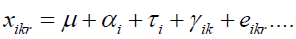 (1)
(1)
With i = 1,2,……………,g, k = 1,2,…………,b and r = 1,2,…………,n and all are p*1 vectors Here,
μ = The grand mean
αi= The treatment effect vector for group i of factor 1
τk= The treatment effect vector for group k of factor 2
eikr = The treatment effect vector for the interaction of group i of factor 1 and group k of factor 2
eikr= The error term
r = The subscript used for observations within each group.
We assume that there are n units in each gb combination of factor levels. The vector of measurements taken on the unit in the treatment group distinguished by the ithlevel of factor 1 and the level of factor 2 can be expressed as
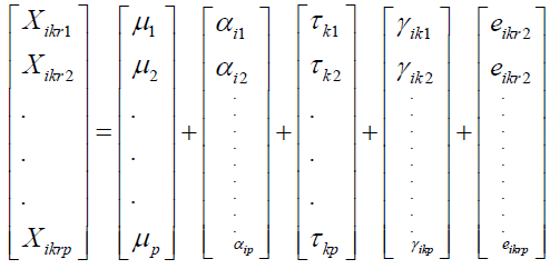 (2)
(2)
Where 
If the interaction effect is non-zero, then the factor effects are not addictive and the effect of one factor depends on the level of the other factor.
 (3)
(3)
Sum of Squares and Cross-Product Matrices
As in the one-factor model, we can decompose the overall variability into different sources. Note that:
 (3)
(3)
where ithis the p*1mean vector of observations at ithlevel of factor 1, iith is the p*1 mean vector of observations at iith level of factor 2 and iith is the p*1 mean vector of observations at the iith level of factor 1 and the k th level of factor 2. Multiplying both sides in the expression above by the corresponding transposed vectors and summing over n ,k, i we get the usual decomposition.
| Source | SS and CP Matrices | Degrees of Freedom |
|---|---|---|
| Factor 1 |  |
g-1 |
| Factor 2 |  |
b −1 |
| Interaction |  |
(g −1)(b −1) |
| Residual |  |
gb(n −1) |
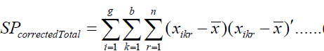
| Corrected Total |  |
gbn −1 |
Where
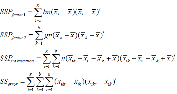
 (4)
(4)
All matrices are p*p dimensional.
Testing Hypothesis in the Two-Way Model Hypothesis of interaction effects
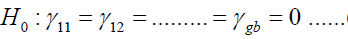 (5)
(5)
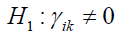
at least for one ik
Wilk’s ∧ statistic has an asymptotic χ2 distribution. For
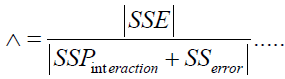 (6)
(6)
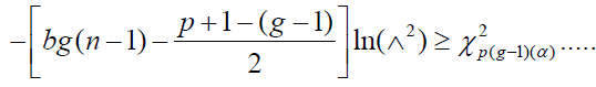
We reject HO at level of α if
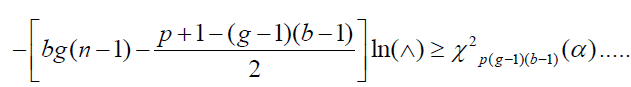 (7)
(7)
A more accurate P-value is obtained from Rao’s F-approximation.
If we fail to reject the null hypothesis of no interaction effects, then we proceed with hypothesis tests for addictive effects of factors 1 and 2 using the appropriate multivariate test statistics.
Hypothesis of no addictivity effect of factor 1
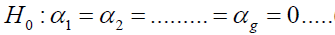 (8)
(8)
at least for one i
The Wilks 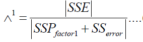 (9) statistic is
(9)
and the null hypothesis is rejected at level 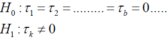 (11)
if
(11)
if
Hypothesis of no addictive effect of factor 2
(11)
atleast for one k
The wilk’s 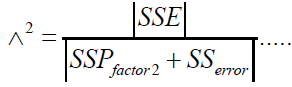 (12)
statistic is
(12)
statistic is
(12)
and the null hypothesis is rejected at level α if
 (13)
(13)
Assumptions
Similar to ANOVA, but extended for multivariate case. The assumptions include:
i) Independence.
ii) Random sampling.
iii) Multivariate normality.
iv) Homogeneity of covariance matrices.
Sample size: The sample size for each levels of the Independent Variable (IV) should not be less than number of levels multiplied by the number of dependent variables.
Equal number of each combination of the levels of each IVs.
i) Linearity.
ii) No outlier.
Post HOC Test (Multiple Comparison Method)
The various methods for multiple-comparisons differ in how well they properly control the overall significance level and in their relative power; some, such as the popular “Duncan’s multiple range test” do not control the overall significance level. For the purpose of this paper, we are going to use Tukey’s Test because it is the best for all-possible pairwise comparisons when sample sizes are unequal or confidence intervals are needed; very good even with equal samples sizes without confidence intervals.
Tukey’s (“Honestly Significant Difference” or “HSD”)
It is based on the distribution of q, the “studentized range.” The “studentized range” with k and r degrees of freedom is the range (i.e., maximum - minimum) of a set of k independent observations from some normal distribution, divided by an independent estimate (with r degrees-of-freedom) of the standard deviation of that normal distribution. Many texts have tables of this distribution.
If there are i samples, all populations’ means are the same (the complete null hypothesis is true),  and are the largest
and smallest sample means, and nS and nS are the respective sample sizes, then:
and are the largest
and smallest sample means, and nS and nS are the respective sample sizes, then:
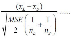 (14)
(14)
It will follow the studentized-range distribution with i and N - i degrees of freedom (N is the total sample size). Critical values
for q then would be appropriate for comparing and
Although other pairs of means do not actually represent the range of the observed sample of means (they will differ by less
than (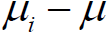 -
- ) q critical values also are used for comparing them; these results in a conservative procedure.
 Confidence Interval for
 is
is
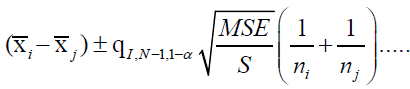 (15)
(15)
μj and μj are significantly different at level α if
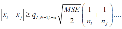 (16)
(16)
Fertilizer type and soil type are the independent variables (IVs) while Crop yield and Crop Height are the dependent variables (DVs). Each of the IVs has equal sample sizes across levels and is categorical while all the DVs are numerical or scale data sets (Table 1).
| Fertilizer Type | Soil Type | Crop Yield(Grams) | Crop Height(CM) |
| Inorganic (NPK) | Loamy | 400 | 32 |
| Inorganic (NPK) | Loamy | 425 | 42 |
| Inorganic (NPK) | Loamy | 367 | 28 |
| Inorganic (NPK) | Loamy | 350 | 22 |
| Inorganic (NPK) | Sandy | 600 | 65 |
| Inorganic (NPK) | Sandy | 580 | 69 |
| Inorganic (NPK) | Sandy | 523 | 60 |
| Inorganic (NPK) | Sandy | 456 | 55 |
| Inorganic (NPK) | Clay | 45 | 19 |
| Inorganic (NPK) | Clay | 64 | 13 |
| Inorganic (NPK) | Clay | 90 | 17 |
| Inorganic (NPK) | Clay | 131 | 21 |
| Organic | Loamy | 600 | 30 |
| Organic | Loamy | 678 | 48 |
| Organic | Loamy | 534 | 66 |
| Organic | Loamy | 324 | 53 |
| Organic | Sandy | 780 | 67 |
| Organic | Sandy | 689 | 63 |
| Organic | Sandy | 456 | 54 |
| Organic | Sandy | 234 | 42 |
| Organic | Clay | 53 | 12 |
| Organic | Clay | 80 | 24 |
| Organic | Clay | 22 | 22 |
| Organic | Clay | 73 | 15 |
Table 1. Shows the data used for illustration.
Entering Data in the SPSS Environment
Launch SPSS version 17 and click the “variable view tab” to see the window here. Since fertilizer_types and soil_types are categorical, we have to recode the values as numbers. Click on values and enter value label entities, click on “Add” to add value labels, then click ok.
Do same for soil_types but this time 1 represent loamy, 2 represents sand and 3 represents clay. Then change their meaure to “nominal” in order to accommodate non numeric values in the data view window (Figure 1).

Figure 1: Entering Data (Variable view)
Entering Data in the SPSS Environment
Launch SPSS version 17 and click the “variable view tab” to see the window here. Since fertilizer_types and soil_types are categorical, we have to recode the values as numbers. Click on values and enter value label entities, click on “Add” to add value labels, and then click ok.
Do same for soil types but this time 1 represent loamy, 2 represents sand and 3 represents clay. Then change their measure to “nominal” in order to accommodate non numeric values in the data view window (Figure 2).

Figure 2: Data view.
Consider the two test statistic for testing normality assumptions (Kolmogorov-Smirnov and Shapiro-Wilk). The p-values of 0.119 and 0.065 for the two tests are not less than 0.01. So, we do not reject the null hypothesis of normality and therefore we conclude that the variable (Crop Yield) follows normal distribution. Also the p-values of 0.164 and 0.022 for the two tests are not less than 0.01. So, we do not reject the null hypothesis of normality and therefore we conclude that the variable (Crop Height) follows normal distribution (Figure 3 and Table 2 and Plot 1).

Figure 3: Normality test.
| Variables | Kolmogorov-Smirnova | Shapiro-Wilk | ||||
|---|---|---|---|---|---|---|
| Statistics | df | Sig. | Statistic | df | Sig. | |
| Crop Yeild in gram | 0.159 | 24 | 0.119 | 0.922 | 24 | 0.065 |
| Crop Height in cm | 0.151 | 24 | 0.164 | 0.9 | 24 | 0.022 |
Table 2: Tests of normality.

Plot 1: Normality plots.
Here we are concerned with the value of the Mahal. Distance value. The critical value for Mahal. Distance is 13.82 when you have two dependent variables. Since Mahal. Distance maximum value of 6.894 is not greater than 13.82 and the univariate normality test is not also significant, then we assume multivariate normality for the dependent variables. Also this test verifies the assumption of no outliers in the dependent variables (Figures 4 and 5, and Table 3).

Figure 4: Mahananobis distance test.

Figure 5: Linearity test procedure.
| Variables | Minimum | Maximum | Mean | Std. Deviation | N |
|---|---|---|---|---|---|
| Mahal. Distance | 0.113 | 6.894 | 1.917 | 1.308 | 24 |
| Cook's Distance | 0 | 0.612 | 0.075 | 0.161 | 24 |
| Centered Leverage Value | 0.005 | 0.3 | 0.083 | 0.057 | 24 |
Table 3: Residuals statistics.
Here we test the assumption of linear relation between each pair of the dependent variable across each level of the independent variables using the matrix dot scatter plot. We are concerned with seeing an elliptical shape starting from the bottom left and moving to the top right in the boxes. Observed that in most cases above, there is such movement, therefore we assume we met the linearity assumption (Figure 6 and Plot 2).

Figure 6: Correlation test procedure.

Plot 2: Matrix dot scatter plot.
Here we test the assumption of multi-collinearity. Correlation is significant at the 0.01 level (2-tailed). This simply implies that there is a significant relationship between the two dependent variables. Since the Pearson Correlation value of 0.841 is not greater than 0.9 but greater than 0.2 we conclude that there is a relationship but not highly correlated. Therefore, these dependent variables are not multi-collinear (Figure 7 and Table 4).

Figure 7: Multivariate analysis procedure (MANOVA method).
| Variables | Crop Yeild(gm) | Crop Height(cm) | |
|---|---|---|---|
| Crop Yeild in grams | Pearson Correlation | 1 | 0.841 |
| Sig. (2-tailed) | 0 | ||
| N | 24 | 24 | |
| Crop Height in cm | Pearson Correlation | 0.841 | 1 |
| Sig. (2-tailed) | 0 | ||
| N | 24 | 24 |
Table 4: Correlations output.
Notice that we met the assumption of sample size provided that 8 is greater than 3*2=6 and 12 is greater than 2 × 2=4. The between-subjects factor shows that we have 2 levels (Inorganic and Organic) of factor one and 3 levels (Clay, Loamy and Sandy) of factor two (Table 5).
| Variables | Value Label | N | |
|---|---|---|---|
| Type of soil where the fertilizer was applied | 1 | Clay | 8 |
| 2 | Loamy | 8 | |
| 3 | Sandy | 8 | |
| Type of Fertilizer used | 1 | Inorganic (NPK) | 12 |
| 2 | Organic | 12 |
Table 5. General linear model with between-subjects factors.
Here, we can see the means for crop yield and crop height for each of the combination of the independent variables. Observe that there is the least average crop yield for the linear combination of organic manure and clay soil. Also the linear combination of inorganic manure and clay soil produced the least crop height. The linear combinations of inorganic and sandy and organic and loamy produced the highest crop yield on average while inorganic and sandy produced the highest crop height on average (Table 6).
| Variables | Type of Soil where the fertilizer was applied | Type of Fertilizer used | Mean | Std. Deviation | N |
|---|---|---|---|---|---|
| Crop Yield in grams | Clay | Inorganic (NPK) | 82.5 | 37.22454 | 4 |
| Organic | 57 | 25.98718 | 4 | ||
| Total | 69.75 | 32.69666 | 8 | ||
| Loamy | Inorganic (NPK) | 385.5 | 33.53108 | 4 | |
| Organic | 539.75 | 245.284 | 4 | ||
| Total | 462.625 | 181.8366 | 8 | ||
| Sandy | Inorganic (NPK) | 539.75 | 64.66516 | 4 | |
| Organic | 534 | 151.8684 | 4 | ||
| Total | 536.875 | 108.1024 | 8 | ||
| Total | Inorganic (NPK) | 335.9167 | 202.9288 | 12 | |
| Organic | 376.9167 | 280.5606 | 12 | ||
| Total | 356.4167 | 240.3733 | 24 |
Table 6. Descriptive statistics output.
The Box’s M test of equality of covariance matrices is not significant at 0.01 alpha level since p-value of 0.103 is not less than 0.01. Therefore, we do not reject the null hypothesis of equal covariance matrices and conclude that there is no significant difference in the covariance matrices of the dependent variables across groups (Table 7).
| Box's M | 58.084 |
|---|---|
| F | 2.752 |
| df1 | 15 |
| df2 | 1772.187 |
| Sig | 0.103 |
Table 7. Box's test of equality of covariance matrices.
Since we did not violate any of the assumptions of the Multivariate Analysis of Variance, we are going to focus on the Wilk’s Lambda test statistics. For information sake, assuming we violated any of the assumptions, then pillar’s trace statistic is more robust. So consider soil type and Wilk’s lambda, the p-value is 0.000 which is a statistically significant value there, so we reject the null hypothesis that the combination of Crop yield and Crop Height is equal for all levels of soil type. The partial Eta squared value tells us the percentage of variation that is explained in crop yield and crop height by soil type. A value of 0.624 indicates that only 62.4% of the variations were explained by soil type. Consider Fertilizer type and Wilk’s lambda, the p-value is 0.494 which is a not statistically significant value there, so we do not reject the null hypothesis that the combination of Crop yield and Crop Height is equal for all levels of Fertilizer type. The partial Eta squared value tells us the percentage of variation that is explained in crop yield and crop height by soil type. A value of 0.08 indicates that only 8% of the variations were explained by fertilizer type. Consider Soil_Type * Fertilizer_Type and Wilk’s lambda, the p-value is 0.21 which is a statistically significant value there, so we reject the null hypothesis that the combination of Crop yield and Crop Height is equal for all levels of Fertilizer type and Soil Type. The partial Eta squared value tells us the percentage of variation that is explained in crop yield and crop height by the linear combination of soil type and fertilizer type. A value of 0.309 indicates that only 30.9% of the variations were explained by the linear combination of fertilizer type and soil type. This simply means that fertilizer type reduces the percentage of variation explained by the interaction effect (Table 8).
| Effect | Value | F | Hypothesis df | Error df | Sig. | Partial Eta Squared | |
|---|---|---|---|---|---|---|---|
| Intercept | Pillai's Trace | 0.964 | 228.82 | 2 | 17 | 0 | 0.964 |
| Wilks' Lambda | 0.036 | 228.82 | 2 | 17 | 0 | 0.964 | |
| Soil_Type | Pillai's Trace | 0.928 | 7.785 | 4 | 36 | 0 | 0.464 |
| Wilks' Lambda | 0.141 | 14.116 | 4 | 34 | 0 | 0.624 | |
| Fertilizer_Type | Pillai's Trace | 0.08 | 0.735 | 2 | 17 | 0.494 | 0.08 |
| Wilks' Lambda | 0.92 | 0.735 | 2 | 17 | 0.494 | 0.08 | |
| Soil_Type * Fertilizer_Type | Pillai's Trace | 0.539 | 3.318 | 4 | 36 | 0.021 | 0.269 |
| Wilks' Lambda | 0.478 | 3.800a | 4 | 34 | 0.012 | 0.309 | |
Table 8. Multivariate tests
Here, we test the null hypothesis that the error variance of the dependent variable is equal across groups. Observe that for crop yield, the p-value of 0.222 is greater than 0.01, the test is not statistically significant. Therefore, we conclude that the error variance of Crop yield is equal across groups and also the error variance for crop heights is not significant since 0.299 is not less than 0.01. We conclude that the error variance is equal across groups (Tables 9-11).
| Variables | F | df1 | df2 | Sig. |
|---|---|---|---|---|
| Crop Yeild in grams | 5.764 | 5 | 18 | 0.222 |
| Crop Height in cm | 1.321 | 5 | 18 | 0.299 |
Table 9. Levene's test of equality of error variances.
| Source | Dependent Variable | Type III Sum of Squares | df | Mean Square | F | Sig. | Partial Eta Squared |
|---|---|---|---|---|---|---|---|
| Corrected Model | Crop Yeild in grams | 1.06E+06 | 5 | 211428 | 14.003 | 0 | 0.795 |
| Crop Height in cm | 7634.375b | 5 | 1526.88 | 18.442 | 0 | 0.837 | |
| Intercept | Crop Yeild in grams | 3048788 | 1 | 3048788 | 201.917 | 0 | 0.918 |
| Crop Height in cm | 36738.4 | 1 | 36738.4 | 443.745 | 0 | 0.961 | |
| Soil_Type | Crop Yeild in grams | 1008186 | 2 | 504093 | 33.385 | 0 | 0.788 |
| Crop Height in cm | 5994.75 | 2 | 2997.38 | 36.204 | 0 | 0.801 | |
| Fertilizer_Type | Crop Yeild in grams | 10086 | 1 | 10086 | 0.668 | 0.424 | 0.036 |
| Crop Height in cm | 117.042 | 1 | 117.042 | 1.414 | 0.25 | 0.073 | |
| Soil_Type * Fertilizer_Type | Crop Yeild in grams | 38866.8 | 2 | 19433.4 | 1.287 | 0.3 | 0.125 |
| Crop Height in cm | 1522.58 | 2 | 761.292 | 9.195 | 0.002 | 0.505 | |
| Error | Crop Yeild in grams | 271786 | 18 | 15099.2 | -- | -- | -- |
| Crop Height in cm | 1490.25 | 18 | 82.792 | -- | -- | -- | |
| Total | Crop Yeild in grams | 4377712 | 24 | ||||
| Crop Height in cm | 45863 | 24 | -- | -- | -- | ||
| Corrected Total | Crop Yeild in grams | 1328924 | 23 | ||||
| Crop Height in cm | 9124.63 | 23 | -- | -- | -- |
Table 10. Tests of between-subjects effects.
| Dependent Variables | (I) Type of Soil | (J) Type of Soil | Mean Difference (I-J) | Std. Error | Sig. | 95% Confidence Interval | |
|---|---|---|---|---|---|---|---|
| Lower Bound | Upper Bound | ||||||
| Crop Yeild in grams | Clay | Loamy | -392.875 | 61.4393 | 0 | -549.678 | -236.0716 |
| Sandy | -467.125 | 61.4393 | 0 | -623.928 | -310.3216 | ||
| Loamy | Clay | 392.875 | 61.4394 | 0 | 236.072 | 549.6784 | |
| Sandy | -74.25 | 61.4394 | 0.464 | -231.053 | 82.5534 | ||
| Sandy | Clay | 467.125 | 61.4394 | 0 | 310.322 | 623.9284 | |
| Loamy | 74.25 | 61.4394 | 0.464 | -82.5534 | 231.0534 | ||
| Crop Height in cm | Clay | Loamy | -25.875 | 4.5495 | 0 | -37.4861 | -14.2639 |
| Sandy | -37.875 | 4.5495 | 0 | -49.4861 | -26.2639 | ||
| Loamy | Clay | 25.875 | 4.5495 | 0 | 14.2639 | 37.4861 | |
| Sandy | -12 | 4.5495 | 0.042 | -23.6111 | -0.3889 | ||
| Sandy | Clay | 37.875 | 4.5495 | 0 | 26.2639 | 49.4861 | |
| Loamy | 12 | 4.5495 | 0.042 | 0.3889 | 23.6111 | ||
Table 11. Multiple comparisons.
Here we are looking for significant findings, So we can see a statistically significance result for soil type on crop yield and crop height. This simply means that soil type plays a significant role on crop yield and crop height. While fertlizer type do not have a significant role to play on crop yield and crop height. The interaction effect is significant for crop height, this implies that the linear combination of soil type and fertilizer type significantly affect the height of the crop. The effect size of soil type on crop yield and crop height is 0.788(78%) and 0.801 (80%). This means that about 78% of variations in crop yield is as a result of the soil type and 80% of the variation in crop height is as a result of soil type too. Only 50% of variation in crop height is explained by the linear combination of soil type and fertilizer type. The corrected models were statistically significant with 79.5% and 83% effect sizes (same as R------=squared values).
Post HOC Tests
Type of soil where the fertilizer was applied.
Tukey HSD
This is the profile plot for crop yield data. It shows that organic manure produced more estimated marginal average crop yield in loamy soil followed by sandy and finally clay soil. Inorganic manure (NPK) produced more estimated marginal estimated crop yield in sandy, followed by loamy and then clay. Across the three levels, that was significant changes in the estimated crop yields (Plot 3).

Plot 3: Crop yield in grams.
This is the profile plot for crop height data. It shows that organic manure produced more estimated marginal average crop height in loamy soil followed by sandy and finally clay soil. Inorganic manure (NPK) produced more estimated marginal average crop yield in sandy, followed by loamy and then clay. As a matter of fact, inorganic manure (NPK) produced more estimated marginal average height in sandy soil than organic manure did. Across the three levels, that was significant changes in the estimated crop heights (Plot 4).

Plot 4: Crop height in cm.
Two-way Multivariate Analysis of Variance (MANOVA) is used when two independent variables both of which contains two or more levels and two or more dependent variables measured on the scale level measurement. The independent variables were soil type (with 3 levels) and fertilizer type (2 levels) while the dependent variables were crop (tiger nut)(tiger nut) yield and crop height. We presumed that all data of the dependent variables are loaded as t-scores. T-scores are standard scores with mean of 50 and standard deviation of 10. We also presumed that all observations were independent. We tested the statistical significant difference between the effects of all levels of soil_ types as well as fertilizer types on the linear combination of tiger nut yield and height. We estimated the effect of the combination of soil type and fertilizer type on the linear combinations of the tiger nut yield and height. We also estimated the main effects of all levels of each of the independent variables on the dependent variables. We observed that soil_type plays a significant role on tiger nut yield and height. While ferlizer_type do not have a significant role to play on tiger nut yield and height. The intearaction effect is significant for tiger nut height, this implies that the linear combination of soil_types and fertilizer_types significantly affect the height of tiger nuts. The effect size of soil_types on tiger nut yield and height is 0.788(78%) and 0.801 (80%). This means that about 78% of variations in tiger nut yield is as a result of the soil_type and 80% of the variation in height is as a result of soil_type too. Only 50% of variation in its height is explained by the linear combination of soil_type and fertilizer_type. The corrected models were statistically significant with 79.5% and 83% effect sizes (same as Rsquared values). We observed that there is the least average tiger nut yield for the linear combination of organic manure and clay soil. Also the linear combination of inorganic manure and clay soil produced the least tiger nut height. The linear combinations of inorganic and sandy and organic and loamy produced the highest yield on average while inorganic and sandy produced the highest height on average. We also saw that organic manure produced more estimated marginal average yield in loamy soil followed by sandy and finally clay soil. Inorganic manure (NPK) produced more estimated marginal estimated yield in sandy, followed by loamy and then clay. Across the three levels, there were significant changes in the estimated yields. organic manure produced more estimated marginal average tiger nut height in loamy soil followed by sandy and finally clay soil. Inorganic manure (NPK) produced more estimated marginal average yield in sandy, followed by loamy and then clay.
Based on the findings of this research, the following recommendations are made;
I. The Researchers need to investigate amongst all the laid out assumptions of MANOVA to verify the possibility of going on with the analysis to avoid misleading results from the analysis. It is unavoidable to have misleading results from data that contains serious outliers and are not multivariate normally distributed.
II. Since soil type played a significant role on crop yield and crop height. While fertilizer type do not have a significant role to play on crop yield and crop height and the intearaction effect is significant for crop height,we recommend that agriculturists should take into serious consideration the soil type where farming activities would take place to have a rewarding crop yield.
III. While we recommend that farming activities be carried out on loamy soil and partly sandy soil, clay soil resulted to be inappropriate for farming activities.
IV. Expect more crop yield and crop height on sandy soil when you applied inorganic manure and more on loamy soil when you apply organic manure.