A Wavelet Analysis for the Relationship between Financial Stress and the Equity Premium in US

Abstract

This study investigates the empirical influence of financial stress on equity premium in the case of United States by using the wavelet transform framework. This new methodology enables the decomposition of timeseries at different time-frequencies. Generally, empirical results show strong evidence of significant linkage between financial stress on the stock markets. These findings confirm that financial stress is majority having the influence over equity premium in short run, but also for both medium and large time horizons.

Keywords

Wavelet analysis, Wavelet coherence, Financial stress, Equity premium, United States.

Introduction

It is well known that the 2007-2008 US subprime financial crisis has strongly affect the rest of the world which turns rapidly into the great recession. Most of the countries have overcome this crisis time period from mid of 2009 but the recovery process prolonged across various countries leading to the appearance of significant financial stress. As advanced by [1], financial stress can be defined as an interruption of the normal functioning of financial markets. One common sign of financial stress is increased uncertainty of the fundamental values of financial assets like stocks. For the stocks, the fundamental values correspond to the present discounted value of the future cash flows including dividends and interest payments. Increased uncertainty regarding these values induces a greater variability in the market prices of the stocks and thus makes higher volatility in the financial market, which into turn leads to bigger uncertainty for future profits and to lower investment spending trend. This claim is supported by several authors like Bloom [2]; Guiso and Parigi [3] and Leahy and Whited [4] who find that financial market volatility increases during financial stress. In the same line Bernanke [5] show that the financial market performs smoothly under low financial stress. Consequently, the transaction between savers and borrowers facilitate the stock market to operate well. More precisely, if financial stress is more stressful, the firms are unable to attract funds from savers and hence volatility increases in the financial sector.

Regarding the literature, the empirical relationship between financial stress and stock market has been extensively examined. Some studies have dealt with the movements of the stock market, considering various predictors and statistical approaches [6-11]. These studies use different estimates, such as stock market returns using macro-economic variables, corporate actions, price multiples, consumer sentiments and risk. In addition, some studies report that the stock market can predict from these factor [12,13] while other studies was failed to forecast stock returns using other variables [14]. On the same context, one study of [15] argued that the behavior of stock market return is explained by specific factors such as information asymmetry, transaction cost and agent heterogeneity (for instance, hedge funds, speculators and long-term investors). Some empirical studies focus on the forecasting behavior of stock market returns. Lewellen [16] and Stambaugh [17] work are the evidence of this argument. Not only this, traders can earn a normal profit against speculation on future prices due to sufficient information available in the asset price [18]. Similarly [13,19] raise a question over spurious estimators of stock market returns. Welch and Goyal [20]; Gupta et al. [14] work also contributed about weak support of stock market return predictors.

In the context of financial distress, the stock market return can be explained using financial stress and economic uncertainty. The predictors are mainly associated with systematic risk and can be significant in order to predict stock market return compared with traditional estimators. So, it is necessary to build a connection between the stock market return and financial conditions as the literature support is inadequate and has not been widely investigated particularly in the US market [15]. In this study, we try to examine the stock market volatility and financial stress for US economy. In this sense, the general asset pricing theory suggests that time varying overall risk and stock market return are key determinants to investigate. Gupta et al. [15] study further emphasized that stock market return is an open issue to further evaluate and investigate. There are several reasons to study the stock market and financial stress, both empirically and theoretically. First, economic indicators are mainly linked with equity prices, whereas it reflects future growth in the stock market. In the US stock market [21], suggest that stock prices were found to be very low in crisis time. Furthermore, corporate investment decisions were also influenced by the decline in equity prices. In addition, stock prices decrease in highly leveraged balance sheets when considering financial sector.

For the case of the US stock market [22], suggest that the mean of 2.5 percent increase in share premium during 1951 to 2000. Siegel [23] uses more historical data, find that, the US stock market premium was 3.9 percent during the sample period of 1871 to 1925 while 3.17 share premium was noted in 1802 to 1870 time period. Jawadi and Arouri [24] highlighted the relationship between subprime financial crisis and US stock market return and find that, US systematic and global risk leads to increase in US stock markt return specifically after the financial crisis. Furthermore, the stock market return or equity premium for developed economies has been a subject of interest for researchers [25-27]. Specifically, equity prices and financial stress have also been studied by earlier studies [21,28-30].

Early stages in predicting stock market return build an interest to propose a theoretical framework that evaluates the stock market excess return. Meese and Rogoff [31] work is an extension of this argument. Recent investigations have contributed more precisely to predict stock return using different approaches, Welch and Goyal [20] applied sum of the parts (SOP) framework while Ferreira and Santa- Clara [14] and Campbell and Thomson [32] proposed a new regression model to predict stock returns. Similarly, Rapach and Zhou [33] suggest parameter instability and model uncertainty in the data generating process. Abou and Part [27] adopted forward and backward approach. French et al.[34], uses ARCH effect, whereas Ameur et al. [35], applied CAPM-GARCH methodology.

The main objective of this paper is to examine the empirical influence of the financial stress (FS) on the equity market premium (EP) for the case of United States over the period from 1990 to 2015 using wavelet techniques. As measure of the financial stress, we consider following Hakkio and Keeton (2009), the Kansas City Fed stock index. The equity market premium is determined by the difference between the stock market return (i.e. the return of S&P 500 total index).

This study has major contribution in the existing body of knowledge to predict the behavior of equity premium under the condition of financial stress in United States. In contrast to the study of Gupta et al. (2014), we have considered a more recent and updated information in the US stock market using newly introduced wavelet-approach in financial markets. Theoretically, the stock market return is a time varying factor. This signifies that stock market may increase (or decrease) during financial stress time period. Our estimations are based on stock market return and financial stress in US stock market under the wavelet based approach. The advantages to use this technique are two-folded. First, this technique uses time-varying and latest data which are not addressed by past literature. Second, we assure to provide a ground for further studies using the wavelet approach in financial markets, which is a unique contribution in existing literature.

The remaining section of the study is presented on the basis of the following outline. Section 2 presents the wavelet methodology and describes the wavelet-based approach. An empirical application is proposed in section 3. Finally, some conclusions are provided in section 4.

A brief note on wavelet approach

Wavelet analysis's applications have reached a wide range of fields, particularly economics and finance. The starting point in such analysis is based on decomposing a time series on a scale-by-scale basis. This theory has its roots in Fourier analysis. Nevertheless, significant differences prevail between the two transforms. As a matter of fact, in order to represent a given function, the Fourier transform uses complex exponential functions which are inherently nonlocal and stretch out to infinity. Conversely, wavelet building blocks are mathematical functions which are defined over a finite domain and possess remarkable localization properties. Besides, the wavelet transform utilizes a basic function (called the mother wavelet), then dilates and translates it to capture the features that are local in time and in frequency and can describe local characteristics of a given signal in a parsimonious way.

The continuous wavelet transform

The continuous wavelet transform is defined as a projection of a specific wavelet onto the examined time series ,

, (1)

where denotes the complex conjugate, u determines the exact position of the wavelet and the scale parameter s controls how the wavelet is stretched or dilated. If the scale is lower (higher), the wavelet is more (less) compressed, therefore the wavelet is able to detect higher (lower) frequency components of the examined time series X(t) .

A wavelet must fulfill the admissibility condition

, (2)

where is the Fourier transform of a wavelet .

The time series X (t) can be reconstructed using the wavelet coefficients as

, (3)

The continuous wavelet transform preserves energy of the analyzed time series

. (4)

The discrete wavelet transform

The Discrete Wavelet Transforms (DWT) is any wavelet transform for which the wavelets are discretely sampled. It is based on two-channel filter bank called a wavelet filter and scaling filter denoted by and, respectively, where is the length of the filter. The wavelet filters (a high-pass filter)and the scaling filters (low-pass filter) satisfying the quadrature mirror relationship given by for l = 0,..., L −1 are used to construct the DWT matrix.

The wavelet and scaling coefficients of a time series X (t) at the j^th level are defined as

, (5)

. (6)

Daubechies (1992) defined a useful class of wavelet filters, namely the Daubechies compactly supported wavelet filters of width the same symbol of L as for example D(L) and distinguishes between two choices - the extremal phase filters D(L) and the least asymmetric filters LA(L) . The Daubechies wavelet has many desirable properties; its most useful property is possessing the smallest support for a given number of vanishing moments³.

Orthogonal discrete wavelet transform (DWT) however, comes with two main drawbacks: the dyadic length requirement (i.e., a sample size divisible by 2 ^j ), and the fact that the wavelet and scaling coefficients are not shift invariant due to their sensitivity to circular shifts because of the decimation operation.

The maximal overlap DWT (MODWT)

An alternative to DWT is represented by a non-orthogonal variant of DWT: the maximal overlap DWT (MODWT). Contrary to DWT, the MODWT does not decimate the coefficients. So, the number of scaling and wavelet coefficients at every level of transform is the same as the number of sample observations. The price of MODWT is loss of orthogonality and computational efficiency, the transform does not have any sample size restriction and is shift invariant. This transform utilizes the rescaled filters and , j = 1,…,J , where J is the total number of levels⁴.Wavelet and scaling coefficients are obtained as follows:

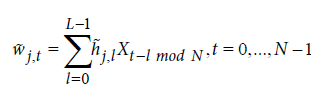, (7)

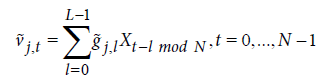. (8)

The non-decimated wavelet coefficients represent differences between generalized averages of data on scale . MODWT comes with all the functions of DWT, but also offers extra benefits. For example, it can handle any sample size, it is translation invariant, as shift in the signal does not change the pattern of wavelet transform coefficients; and provides increased resolution at coarser scales. In addition, MODWT provides a larger sample size in the wavelet correlation analysis and produces a more asymptotically efficient wavelet covariance estimator than the DWT. For a more detailed introduction to wavelets [36,37].

The wavelet analysis of coherence and phase spectra

Since we study the interactions between two time series, we introduce a bivariate setting called wavelet coherence. The cross wavelet transform of two time series (X (t),Y (t)) is defined as

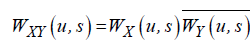, (9)

where W_X (u, s) and W_Y (u, s) denote the continuous wavelet transforms of X (t ) and Y (t ) , respectively, u defines a time position, and s denotes the scale parameter. Thus, the cross wavelet power is obtained via W_XY (u, s) represents the local covariance between the examined time series at the specific scale u. In other words, it indicates where the time series have high common power in the time-frequency domain. Following Torrence and Webster [38], we define the squared wavelet coherence coefficient as follows

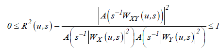, (10)

where A is a smoothing operator in both time and scale which is essential in coherence analysis⁵. Otherwise the ratio R(u,s) would be equal to one. The squared wavelet coherence can be perceived as a local linear correlation between two time series at a particular scale. To distinguish between negative and positive correlation, we use the wavelet coherence phase differences which indicate delays in the oscillation between the two examined time series. We test statistical significance of the wavelet coherence estimates using Monte Carlo methods. The testing procedure is based on the approach of Grinsted et al [39]. and Torrence and Compo [40].

The delay in the oscillation between two time series at some specific time and scale can be obtained by evaluating the wavelet coherence phase difference. Following Torrence and Webster, the wavelet coherence phase differences is defined as

. (11)

where and are the real and the imaginary parts of the smoothed cross wavelet transform.

A phase-difference of zero indicates that the time-series move together at the specified frequency. If then the series move in phase, but the time series Y leads to X . If then it is X that is leading. A phase-difference of π or (−π ) indicates an anti-phase relation. If then X is leading. Time-series Y is leading if.

Empirical Results

As stated earlier, the objective of this research is to analyze the impact of financial stress (FS) on equity premium (EP) in the case of United States. The data for financial stress is gathered from the Kansas City Fed’s financial stress index. The equity market premium in the US is measured as the difference between the return on the S&P 500 total return index and the return on a risk free three month treasury bills. The data for S&P 500 index and treasury bills is collected from Datastream. We have a sample of N=301 monthly observations from 1990(4) to 2015(4). The data is converted in the logarithmic difference series in order to obtain the return-series to make our findings more comparable. In Figure 1 we plot the difference time series of FS and EP for United States.

Figure 1: Real difference series of FS and EP for United States.

We can see the significant fluctuations in the real difference series of both variables FS and EP. We can see the significant fluctuations in the real difference series of both variables FS and EP from the period of 2008 financial crisis. These findings confirm that in monthly observations there are important changes in both series throughout the sample. We use wavelet based unit root test by Fan and Gencay [41], Augmented Dickey Fuller (ADF)⁶ and Phillips and Perron (PP)⁷ unit roots tests to judge the stationary properties of both series FS and EP. Results of unit root tests are reported in Tables 1 and 2. Results of all three unit root tests suggest that the series of FS and EP are non-stationary at level, but they become stationary at first difference. These findings suggest that there is no issue of unit root problem in our both variables. Further, we estimate the long run relationship between financial stress and equity premium by using the two co-integration methods namely, Autoregressive distributed lag (ARDL) method8 for cointegration and Johansen and Juselius [44] cointegration method. The experiential equation of the ARDL model is given below.

Table 1. Stationary Test Results.

Table 2. Wavelet based unit root tests.

(12)

where ψ₀ is a constant while, μ_t is a white noise error term. The error correction dynamic is taken by the variables related with the summation symbols, whereas the other part of the equation indicates the long run relationship. Schwarz Bayesian Criteria (SBC) is taken to examine the optimum and maximum numbers lags of the model and all series. The Johansen and Juselius cointegration technique is constructed on λ _trace and λ_max statistics. The main statistics are assumed by:

(13)

(14)

where the null hypothesis is r = g beside the alternative hypothes is r > g , g = 0,…,n . The null hypothesis in the Johansen and Juselius [40] cointegration test is that there is no long run relationship exists between the variables. Tables 3 and 4 presents the results of ARDL and Johansen and Juselius co-integration methods. Results of both tests indicate that there is a significant relationship exists in between financial stress and equity premium in United States. Now, we move to analyze the relationship between FS and EP through wavelet analysis, after confirming the valid cointegration between both considered variables.

Table 3. J. J. Cointegration test results of Equity Premium Model.

Table 4. Lag Length Selection & Bound Testing for Cointegration.

Discrete wavelet decomposition

In the datasets of different variables there are many periods, and not just the two can represents the appropriate time scales in the particular analysis. Consequently, to study the relationship between FS and EP we use time frequency based approach “Wavelets” to study the different time horizon in the time series. Wavelets consider the problem of non-stationarity as an intrinsic property of data rather than a problem to be solved by the pre-processing of the data. Figures 2 and 3 illustrate the multi-resolution analysis (MRA) of order J = 6 for the FS and EP by using the MODWT based upon the Daubechies [35] least asymmetric ( LA ) wavelet filter. In both above discussed figures we plot the orthogonal components (D₁,D₂, . . .,D₆ ) to show the different frequency components of the original series in details and a smoothed component ( S₆ ). Results show that the high frequencies are found in the short period of both series. Moreover, the variation in the both series is become more stable in the longer periods.

Figure 2: MODWT decomposition of EP on J=6 wavelet levels.

Figure 3: MODWT decomposition of FS on J=6 wavelet levels

Table 5 presents the energy explanation of FS and EP at each scale by using the MODWT. We discuss all movements by making the four major periods, namely; short run (D1), medium run (D2+D3), long run (D4+D5) and very long run (D6+S6). Results indicate that in both FS and EP series the short and medium run explains the most of the variance of around 85% and 99% respectively. The variance of 95% in EP is occurs in the period of first 8 months.

Table 5. Energy Decomposition for the FS and EP.

Continuous wavelets analysis

The continuous wavelet analysis is comparatively easier to interpret as compare to MODWT because it is provide more visible frequency information. Therefore, to ascertain the findings of MODWT we also use continuous wavelet analysis on the relationship of FS and EP. Figure 4 presents the continuous wavelet power spectrum of both series.

Figure 4: Continuous Wavelet power spectra of the EP and FS.

The continuous wavelet power spectrum shows the movements of the series in a three dimensions contour plot: time, frequency and color code. Results indicate that in the case of EP we observe comparatively a quite stable variance up to 2007 in all scales. We also observe the strong variance for the small and medium scale from 2007 to 2015, especially in the period of global financial crisis. Results indicate that in the case of FS we again observe a significant high variance from 2005 to 2012 in the short, medium and long run. These findings suggest that the US economy was under financial stress before the start of financial crisis of 2008. Results also indicate it take around 4 years to prevail over the financial crisis of 2008.

Wavelet Coherence transform

We use wavelet coherence transform to identify the presence of cause and effect relationship between FS and EP in United States. Figure 5 presents the wavelet coherence power spectrum between FS and EP.

Figure 5: Wavelet Coherrence between FS and EP.

First we discuss the findings of short run; we observe the several different situations of significant in-phase and out-phase relationship, but either FS is leading or lagging is not clear. In the medium run, we observe the in-phase relationship between FS and EP from 1998-2003 and in 2012, where FS is leading (FS has a causal influence over EP). We also observe the anti-phase situation from 2005-2009, but the FS is again leading here. In the long run, we only see only valid significant anti-phase situation from 2002-2008, where FS is again leading. These findings of wavelet coherence approach confirm that FS is majority having the influence over EP in short, medium and long run.

Wavelet-Granger causality test

We use wavelet based Granger causality analysis by using the time frequency band of wavelet transform (MODWT) to analyze the causal relationship between financial stress and equity premium. Table 6 presented the results of Granger causality across frequency ranges and time-scales.

Table 6. Results of Wavelet based Granger causality test at different time scales.

The Granger causality test based on MODWT provides us the opportunity to analyze that either FS cause the change in high, medium and low frequencies of the EP series. The empirical results of Table-6 indicate that the raw series of financial stress has unidirectional influence over the raw series of equity premium in United States. Results also show the unidirectional causal relationship between FS and EP in short and medium run which runs from financial stress to equity premium. Results further indicate that there is no causal relationship exists in between FS and EP in the long and very long run. These findings are consistent with the findings of wavelet correlation, and wavelet coherence transform.

Conclusion

In this work, we have considered the wavelet transform framework to analyze the causal relationship between financial stress and equity premium in United States. This new methodology enables the decomposition of time-series at different timefrequencies and provides the specific results for the different time-frequencies based on short, medium, long and very long run. Furthermore, we have used maximal overlap discrete wavelet transform (MODWT), continuous wavelet power spectrum, wavelet coherence spectrum and wavelet based granger causality analysis to analyze the relationship between financial stress and equity premium in United States by using the monthly data from the period of 1990(4) to 2015(4).

The empirical results of ARDL and Johansen-Juselius cointegration show the significant evidence of long run relationship between financial stress and equity premium in United States. However, the results of continuous wavelet indicate that in the case of EP we see strong variance for the small and medium scale from 2007 to 2015. In addition, the results indicate that in the case of FS we again observe a significant high variance from 2005 to 2012 in the short, medium and long run. The results obtained suggest that the US economy was under financial stress before the start of financial crisis. Moreover, the wavelet coherence analysis show that in short run, we observe the several different situations of significant in-phase and out-phase relationship, but either FS is leading or lagging is not clear. These findings of wavelet coherence approach proved that FS is majority having the influence over EP in short, medium and long run. Besides, the results of wavelet based Granger causality analyses indicate that the raw series of financial stress has unidirectional influence over the raw series of equity premium in United States. The results also show the unidirectional causal relationship between FS and EP in short and medium run which runs from financial stress to equity premium. The results further indicate that there is no causal relationship exists in between FS and EP in the long and very long run.

Due to the results obtained, we can conclude a strong influence of the financial stress on the equity premium at different time scales.

¹The wavelet function (filter) of support L∈N proceeds as a special filter possessing specific properties, such that (i) it integrates to zero, i.e., , (ii) has unit
energy, i.e., and (iii) is orthogonal to its even shifts, i.e.,.

²The scaling filter of support L is defined so as to satisfy the following properties, (i) , (ii) and (iii).

³For Daubechies wavelets, the number of vanishing moments is half the filter length.

⁴The MODWT filters satisfies the following properties, (i) , (ii), (iii) and (iv).

⁵Smoothing is achieved by convolution in both time and scale; see Grinsted et al. [40] for more details.

⁶See, Dicky and Fuller [42].

⁷See, Phillips and Perron [43].

⁸See, Pesaran and Pesaran [45], Pesaran and Shin [46] and Pesaran et al. [47,48].

References

1. Hakkio CS and Keeton WR. Financial stress: what is it how can it be measured and why does it matter?” Federal Reserve Bank of Kansas City Economic Review second quarter. 2009.
2. Bloom N. The impact of uncertainty shocks. Econometrica. 2009; 773: 623-685.
3. Guiso L and Parigi G. Investment and Demand Uncertainty. Quarterly Journal of Economics. 1999. 114:185-227.
4. Leahy JV and Whited TM. The Effect of Uncertainty on Investment: Some Stylized Facts Journal of Money Credit and Banking. 1996; 28: 64-83.
5. Bernanke BS. et al. The financial accelerator in a quantitative business cycle framework. Handbook of macroeconomics. 1999; 1: 1341-1393.
6. Boudoukh J. et al. The myth of long-horizon predictability. Review of Financial Studies. 2008; 21: 1577-1605.
7. Ang A and Bekaert G. Stock return predictability: Is it there? Review of Financial studies. 2007; 20: 651-707
8. Alves C. et al. Do stress tests matter? A study on the impact of the disclosure of stress test results on European financial stocks and CDS markets. Applied Economics. 2015; 47: 1213-1229.
9. Gupta R and Modise MP. South African stock return predictability in the context data mining: the role of financial variables and international stock returns. Economic Modelling. 2012; 29: 908-916.
10. Rapach DE and Wohar ME. Valuation ratios and long-horizon stock price predictability. Journal of Applied Econometrics 2005; 20: 327-344.
11. Avramov D. Stock return predictability and model uncertainty. Journal of Financial Economics. 2002; 64: 423-458.
12. Campbell JY. Asset prices consumption and the business cycle.Handbook of macroeconomics. 1999; 1: 1231-1303.
13. Campbell JY. Asset pricing at the millennium. The Journal of Finance. 2000; 55: 1515-1567.
14. Ferreira MA and Santa-Clara P. Forecasting stock market returns: The sum of the parts is more than the whole. Journal of Financial Economics. 2011; 100: 514-537.
15. Gupta R. et al. Can economic uncertainty financial stress and consumer sentiments predict US equity premium?. Journal of International Financial Markets Institutions and Money. 2014; 367-378.
16. Lewellen J. Predicting returns with financial ratios. Journal of Financial Economics. 2004. 74: 209-235.
17. Stambaugh RF. Predictive regressions. Journal of Financial Economics. 1999; 543 375-421.
18. Fama EF. Efficient capital markets: A review of the theory and empirical work Journal of Finance. 1970; 25: 383-420.
19. Ferson W. et al. Is stock return predictability spurious. Journal of Investment Management. 2003. 1: 1-10.
20. Welch I. and Goyal A. A Comprehensive look at the empirical performance of equity premium prediction The Review of Financial Studies. 2008; 24: 1455-1508.
21. Aizenman J and Pasricha GK. Determinants of financial stress and recovery during the great recession International Journal of Finance and Economie. 2012; 17: 347-372.
22. Fama EF and French KR. The equity premium Journal of Finance. 2010; 57: 637-659.
23. Siegel JJ. Perspectives on the equity risk premium. Other Publications 2005; 202-217.
24. Jawadi F and Arouri MH. The current international financial crisis in 10 questions: some lessons. Applied Economics Letters. 2012. 18: 279-283.
25. Pastor L and Stambaugh RF. Liquidity risk and expected stock returns No. w8462. National Bureau of Economic Research. 2001.
26. Siegel JJ and Thaler RH. Anomalies: The equity premium puzzle. The Journal of Economic Perspectives. 1997; 191-200.
27. Abou A and Prat G. The dynamics of US equity premia: lessons from professionals' view. Bankers Markets and Investors. 2010; 104: 4-20.
28. Frankel JA and Saravelos G. Are leading indicators of financial crises useful for assessing country vulnerability? Evidence from the 2008-09 global crisis NBER working paper. 2010.
29. Berkman H. et al. Sell on the news: Differences of opinion short-sales constraints and returns around earnings announcements Journal of Financial Economics. 2009; 92: 3376-399.
30. Rose AK and Spiegel MM. Cross-country causes and consequences of the 2008 crisis: International linkages American exposure Pacific Economic Review. 2010; 15: 340-363.
31. Meese RA and Rogoff K. Empirical exchange rate models of the seventies: Do they fit out of sample? Journal of International Economics. 1983; 14: 3-24.
32. Campbell JY and Thomson SB. Predicting excess stock returns out of sample: Can anything beat the historical average? Review of Financial Studies. 2008; 21: 1509-1531.
33. Rapach D and Zhou G Forecasting stock returns. Handbook of Economic Forecasting 2Part A 2013; 328-383.
34. French KR et al. Expected stock returns and volatility. Journal of financial Economics. 1987; 19: 3-29.
35. Ameur HB. et al. Measuring time-varying equity risk premium in the context of financial crisis: do developed and emerging markets differ? Applied Economics Letters. 2013; 20: 1673-1677.
36. Daubechies I. Ten Lectures on Wavelets. SIAM Philadelphia. 1992.
37. Percival DB and Walden AT. Wavelet Methods for Time Series Analysis. Cambridge University Press Cambridge. 2000.
38. Torrence C and Webster PJ. Interdecadal changes in the enso-monsoon system. Journal of Climate 1999; 12: 2679-2690.
39. Grinsted et al. Application of the cross wavelet transform and wavelet coherence to geophysical time series. Nonlinear Processes in Geophysics.2004; 11: 561-566.
40. Torrence C and Compo GP. A practical guide to wavelet analysis. Bulletin of the American Meteorological Society.1998; 79: 61-78.
41. Fan Y and Gençay R. Unit root tests with wavelets. Econometric Theory 26 1305-1331.
42. Dicky DA and Fuller WA. Distribution of the Estimators for Autoregressive Time Series with a Unit Root. Journal of the American Statistical Association. 1979; 74: 427-431.
43. Phillips PB and Perron P. Testing for a Unit Root in Time Series Regression. Biometrika 1988; 75: 335-346.
44. Johansen S and Juselius K. Maximum Likelihood Estimation and Inference on Cointegration with Applications to the Demand of Money. Oxford Bulletin of Econometrics and Statistics. 1990; 169-210.
45. Pesaran MH and Pesaran B. Working with Microfit 4.0: interactive econometric analysis. Oxford University Press Oxford. 1997.
46. Pesaran MH and Shin Y. Generalized impulse response analysis in linear multivariate models. Economic Letters. 1998; 58: 17-29.
47. Pesaran MH et al. Structural analysis of vector error correction models with exogenous I1 variables. Journal of Econometrics. 2000; 97: 293-343.
48. Pesaran MH et al. Bounds testing approaches to the analysis of level relationships. Journal of Applied Economics. 2001; 16: 289-326.