Keywords
|
| Beam forming, Time Difference of Arrival (TDOA), Direction of Arrival (DOA), Cross Correlation |
INTRODUCTION
|
| People are generally able to discern the direction that a sound is coming from using two ears. The combination of the slightly different signals that arrive at the ears enables us to deduce, intuitively, the direction of the sound. Similarly, a biologically inspired sound localization system can be built by making use of an array of microphones, which are hooked up to a computer. In addition, such a system of microphones can be made to extract any particular sound from a mixture of sounds produced simultaneously by several sources. The spatial location of a sound source can be determined based on multiple observations of the emitted sound signal. The mathematical details of these applications are basically variations of a triangulation scheme, using multiple sensors, which detect a signal emitted by the source that is to be localized, or by using multiple emitters, whose signals are sensed by the sensor (e.g. GPS receiver).The most representative methods frequently used in conjunction with sound source localization are intensity difference between microphones, Beam forming and Time Difference of Arrival (TDOA). In this current work, the phase information present in signals and the Direction of arrival (DOA) of the signals at the microphone arrays are used to find an estimate of the source location. |
ACOUSTIC SOURCE LOCALIZATION
|
| The process of determining the location of an acoustic source relative to some reference frame is known as acoustic source localization. Acoustic source present in the near-field can be localized with knowledge of the time difference of arrivals (TDOAs) measured with pairs of microphones. The speed of sound in the medium in which the acoustic source is present is known. With continued investigation over the last two decades, the time delay estimation (TDE) based localization has become the technique of choice. |
| A. Time Difference of Arrival |
| Time-Delay Estimation (TDE), which aims at measuring the relative time difference of arrival (TDOA) among spatially separated sensors, has played an important role in radar, sonar, and seismology for localizing radiating sources. |
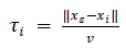
| Suppose the source is emitting a sound signal S(t), and a two-microphone array is observing signals X1(t) and X2(t). The signal received by the microphones will be distorted due to both the acoustics of the room and the ambient noise in the environment. Furthermore, due to the distance between the two microphones in the array, there will be a measurable time difference between observations of the signal at each microphone. This is referred to as the time difference of arrival (TDOA) ,τ , between the microphones. The time τi of a signal S (t) is the amount of time required for a signal to propagate from the source to the ith microphone in an array. |
 (2.1) (2.1) |
| Where xs and zi are the spatial positions of the source and the ith microphone, and ν is the speed of sound in air (m/s). As the sound wave travels through different paths to reach spatially separated microphones, the signal from the source reaches the microphones at different instants of times. The TDOA for a given pair of microphones and the source is defined as the time difference between the signals received by the two microphones. It is computed using the spatial positions of the source and microphone. |
| In figure 2.1, ti is the time taken by the signal to reach microphone i while tj is the time taken by the signal to reach microphone j. The Time Difference of Arrival between the ith and jth microphone when the source ‘S’ is excited is given by TDOA i j . |
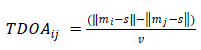 (2.2) (2.2) |
| A TDOA estimate can be obtained by finding the 'τ' that maximizes the cross correlation between the two microphone signals. TDOA’s are then converted to path differences and angle of arrivals. |
| B. Direction of Arrival |
| When the microphones are spatially separated, the acoustic signals arrive at them with differences in time of arrival. From the known array geometry, the Direction of arrival (DOA) of the signal can be obtained from the measured time-delays. The time-delays are estimated for each pair of microphones in the array. Then the best estimate of the DOA is obtained from time-delays and the array geometry. |
| In figure 2.2 receivers 1 and 2 consists of a pair of sensors m1 and m2 which are placed along the X and Y axes respectively. Signals coming from source S, reach the receiver 1, at an angle θ1 with respect to line perpendicular to X- axis. In receiver 1, the extra distance travelled by source signal to reach m1 as compared to m2 will be dcosθ. |
| C. Cross Correlations |
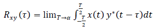
| Cross correlation is a routine signal processing technique that can be applied to find the time delays between two copies of a signal registered at a pair of microphones. The cross correlation between two signals is the measure of similarity between one signal and time delayed version of another signal. Cross correlation between two signals explains how much one signal is related to the time delayed version of another signal. The cross correlation between two signals x(t) and y(t) is defined as |
 (2.3) (2.3) |
| Where 'τ' is called the delay parameter. Cross correlation represents the overlapping area between the signals and the delay parameter determines the maximum possible correlation between two signals. |
SYSTEM DESCRIPTION
|
| A method is proposed to localize an acoustic source within a frequency band from100Hz to 4 kHz in two dimensions using microphone array by calculating the time difference of arrival (TDOA) of the acoustic signals. The Time Difference of Arrival (TDOA) is estimated from the captured audio signals. In this paper, Time difference of arrival (TDOA) based source localization is done based on a two-step procedure. The first stage involves estimation of phase difference between the signals reaching the receivers using the time delay estimation techniques. The estimated phase differences are then transformed into range difference measurements between sensors and the direction of arrival (DOA) of the signal is computed. The range difference or the path difference can also be calculated by directly from the time delay using cross correlation methods. The second stage utilizes efficient algorithms to calculate the location of the source by using the angle of arrival of the signals. |
| A. Assumptions |
| The following conditions are assumed under which location of sound source is estimated: (1) Single sound source is present, which is omni-directional and infinitesimally small. (2) Reflections from the bottom of the plane and from the surrounding objects are negligible. (3) No disturbing noise sources are contributing to the sound field. (4) The source to be located is assumed to be stationary during the data acquisition period. (5)Microphones are assumed to be both phase and amplitude matched and without self noise. The positions of acoustic receivers are known. (6) The change in sound velocity due to change in pressure and temperature are neglected. The velocity of sound in air is taken as 330m/sec. (7) If the distance between the source and the receivers is greater than the distance between the two receivers the sound waves reaching the receivers can be considered to be planar rather than spherical. |
| Figure 3.1 shows the block diagram of the system description. The acoustic signal which is a physical signal is converted into an electrical signal using a transducer. Microphone is an acoustic to electric transducer or sensor that converts sound into an electrical signal. An amplifier is used for increasing the power of an electric signal by use of an external energy source. The dynamic range of an amplifier decides the output levels of an ADC. Filters play a key role in virtually all sampled data systems. Most analog to digital converters (ADCs) are preceded by a filter which removes frequency components that are beyond the ADC's range. In a sampled data system, frequency components greater than half the sampling rate shifts into the frequency band of interest. An anti-aliasing filter is used before a signal sampler, to restrict the bandwidth of a signal to approximately satisfy the sampling theorem. Anti aliasing Filter, is designed to minimize aliasing effects while the required signal is sampled. An analog-to-digital converter (ADC) is a device that converts a continuous signal to a discrete time representation in digital form. The frequency on which the sampling will occur is called sampling rate. The sampling rate should be at least twice the maximum frequency component of the signal of interest. The maximum frequency of the input signal should be less than or equal to half of the sampling rate. The digital output will be a two's complement binary number that is proportional to the input. |
SIGNAL DETECTION AND SOURCE LOCALIZATION
|
| From the different signals reaching the receivers, the signals of sufficient magnitudes and those coming within the specified frequency range are considered for source localization. Power Spectral estimation techniques are employed in the digitized signal to detect the source in spectral domain. The power density spectrum of a signal shows the distribution of power of a signal among the various frequency components. |
| To perform frequency analysis on a discrete time signal the signal is converted to its equivalent frequency domain representation, which is given by the Fourier Transform of the signal. Using FFT, the magnitude of the signal and its corresponding frequency can be found. The signals whose power spectrum crosses a certain limit and that comes in the specified frequency range are considered for source localization. Observing the power spectrum of the signals, the frequency at which the sharp peaks occur can be calculated by the equation, |
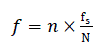 (4.1) (4.1) |
 |
| A. Phase Difference Computation |
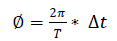
| The signals reaching the microphones at different instants of time will also be having a phase difference between them. Let sin(wt) and sin(wt + Ø) are two signals reaching the receivers. Product of these signals will be, |
 (4.2) (4.2) |
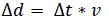
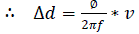
| An FIR filter can be used to filter out the ac components. The remaining part provides the phase difference 'Ø' between the two signals. The phase differences between the signals can be used to obtain the time difference of arrival (TDOA). The difference in the propagation delay and the acoustic velocity in air are known. From this the path difference of the acoustic waves and the direction of arrival (DOA) with respect to the microphone pair can be found. |
 (4.3) (4.3) |
 (4.4) (4.4) |
 (4.5) (4.5) |
 (4.6) (4.6) |
 (4.7) (4.7) |
 (4.8) (4.8) |
 |
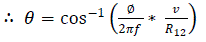
| Hence by calculating the phase difference of two signals the angle of arrival or the direction of arrival (DOA) 'Ø' can be obtained. A microphone pair is coupled with the existing pair of microphones to obtain another value of the direction of arrival. Source location can be estimated using these angles assuming source is in two-dimensional plane. |
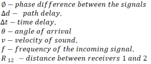
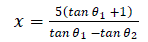
| B. Source Location Estimation |
| Microphones are placed in an L shaped array with a distance of d between the adjacent sensors. Receiver 1 is placed at X- axis with co-ordinates (5,0) and receiver 2 is placed at Y axis having co-ordinates(0,5). If Ø1 is the angle of arrival of the signal at the first receiver and Ø2 is the angle of arrival at the second receiver, the two dimensional location of source (x, y) is given as |
 (4.9) (4.9) |
 (4.10) (4.10) |
EXPERIMENTAL DETAILS
|
| Initially the scenario is created using MATLAB and the source location is computed in two dimensions from the phase difference and cross correlations of the signals arriving at the sensors. Secondly Cross-correlation methods are employed to calculate the time delay of the signals and using this value the angle of arrivals are computed. |
| A. Simulation Results |
| The signals reaching the two receivers are artificially stimulated in a MATLAB environment assuming a sampling frequency of 10000Hz and signal frequency varying from 100Hz to 4 kHz. By cross-correlating and finding the mean value, the phase difference between the signals are computed and the path delay is found. From the path delays direction of arrival (DOA) and location of source is estimated in two dimensions using the equation (4.9) and equation (4.10), assuming the receivers are placed in an L shaped array at known locations |
| The following table shows the values obtained by stimulating the environment in MATLAB. The measured phase differences of signals reaching receivers 1and 2 (ph diff1) and receivers 3 and 4 (ph diff2) are shown. From these the angle of arrivals and source location estimates are obtained. The experiment was carried out for various signal frequencies from 100Hz to 3 kHz and the results for 100Hz and 2200Hz is shown here. |
| Hence by computing the phase difference between the signals arriving at the sensors which are spatially separated, it is possible to find the angle of arrivals and the location of the source. But while computing the location estimates using the phase difference between the signals reaching arrays, ambiguity arises when the frequency exceeds 3.3 KHz. If 'd' is the distance between the two sensors of a receiver, to avoid ambiguity |
 (6.1) (6.1) |
 |
| For a distance of 1m between the sensors, the maximum frequency that provides a unique solution to direction of arrival comes around 3.3KHz. For frequencies above 3.3 KHz the measured phase differences will be ambiguous. Hence 3.3 KHz has to be kept as the upper cut off frequency while finding the source location using phase difference computation in MATLAB. |
| This disadvantage is overcome by cross-correlating the signals in real time. As cross correlations have no frequency constraints, by cross-correlating the signals reaching the receivers the time delay between the signals can be found. The lag at which the cross-correlation function has its maximum value is taken as the time delay between the two signals. From the time delay of the signals, angle of arrival is computed. |
| B. Real Signal Experiments |
| The real signal experiments are carried out using python programming language in real time and the signals are detected using a pair of microphones. PC sound card is used to acquire the signals from the microphones. The captured signals are processed inside the PC and the digitized signals are used for source localization. Figure 5.2 shows the data flow diagram by which the angles of arrival of the signals are computed. The dominant frequencies present in the detected signals are selected from the maximum components of the Fast Fourier Transform (FFT) results. When the power spectrum of the signals crosses a certain limit, these dominant frequencies are detected. The envelope areas of the detected signals are cross correlated taking a portion of signals arriving at a time. From cross-correlation the time delay of arrival between the detected signals is found and substituted in the equations (5.2) and (5.3) to find the direction of arrival (DOA) of the detected signals |
| From Cross correlations the time delay is obtained in terms of number of samples (Δn). Time Delay is given as, |
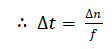 (5.2) (5.2) |
| Using equations (2.3) and (4.5), Direction of Arrival (DOA) of the signals is given as |
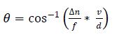 (5.3) (5.3) |
| C. Results Based On Real Time Signals |
| During measurement, the source is kept stationary and at known positions with respect to the sensors. Experiments were done using a pair of microphones which are kept at a spacing of 1m. Velocity of sound is 330m/sec. Hence the worst time delay at which the signals reach the receivers can be 3milliseconds. The signals are sampled in real time at a sampling rate of 44.1 kHz. The time delay in msec and the angle of arrival of the signals are obtained from the peak value of the cross correlated signals using equations (6.2) and (6.3) keeping the source at various locations. |
| From the values obtained the variation in samples of delay and time delay with respect to each positions are plotted. Comparing the values obtained it is found that the time delays for positions 45 degrees and 90 degrees are minimum. At 90 degrees the signals are reaching the receivers almost at the same time and so the Time Difference of Arrival of the signals at 90 degrees is reduced to a minimum. |
CONCLUSION
|
| A number of complications limit the potential accuracy of the system. Some of these are due to physical phenomena that can never be corrected, and others are due to inherent errors built into the processing, due to the design of the system. The error in DOA estimation can be reduced with increase in frame size of signal acquired. Increase in number of frequency components may also improve the DOA estimation. |
| |
Tables at a glance
|
 |
|
|
|
| Table 1 |
Table 2 |
Table 3 |
Table 4 |
|
| |
Figures at a glance
|
 |
 |
 |
 |
 |
| Figure 2.1 |
Figure 2.2 |
Figure 3.1 |
Figure 5.2 |
Figure 5.4 |
|
| |
References
|
- Bob Mungamuru And Parham Aarabi, Enhanced Sound Localization, IEEE Transactions On Systems, Man, And Cybernetics – Part B:Cybernetics, VOL. 34, NO. 3, pp.1526-1540, Jun 2004
- Ashok Kumar Tellakula, Acoustic Source Localization Using Time Delay Estimation, Supercomputer Education And Research Centre Indian Institute of Science, Thesis Report, pp. 1-82, Aug 2007
- Ying Yu And Harvey F. Silverman, An Improved TDOA Based Location Estimation Algorithm For Large Aperture Microphone Arrays, IEEE Explore pp. 77-80,Sept 2009
- Beom-Cheol, Park Keun, Chang Kwak, Kyu-Dae Ban And Ho- Sub Yoon Computer Software And Engineering Human Robot Interaction Team, University Of Science and Technology Intelligent Robot Research Division Korea, Sound Source LocalizationBased On Audiovisual Information for Intelligent Service Robots, Proceeding IEEE International Workshop in Robot and Human Interactive Communication,Dec 2002
- Micheal Shapiro Brandstein, Ph.D, Brown University S.M.E.E Massachusetts Institute Of Technology, A Frame Work For Speech Source Localization Using Sensor Arrays, Thesis Report, May 1998
- Jingcho Chen, Jacob Benesty and Yiteng Huang, Time Delay Estimation Using Spatial Correlation Technique, International Workshop on Acoustic Echo Noise and Noise Control , Kyoto, Japan pp. 207-210 Sept 2003
|