Keywords
|
| Gene expression microarray data, proximity measures, Intrinsic biological separation ability |
INTRODUCTION
|
| The DNA microarray technology has now made it possible to concurrently monitor the expression levels of thousands of genes during important biological processes and across collections of related samples.In elucidating the patterns unseen in gene expression data, it offers a great opportunity for an improved understanding of functional genomics. However, the large number of genes and the complexity of biological systems greatly increase the challenges of understanding and inferring the resulting mass of data, which often consists of millions of measurements. A first phase toward addressing this challenge is the use of clustering techniques. Clustering has two major applications, depending on the type of microarray experiments under analysis. The first is found when expression of genes is monitored across time for a biological process of interest. In the so-called time course experiments, clustering may help, for instance, to identify genes that share the same regulatory mechanisms or functions. The second application involves the analysis of biological samples, usually from different types of cancer |
| The choice of anacceptable proximity measure (similarity or distance) utilized among object pairs is commonlythought to be a fundamental issue in cluster analysis. In spite of the big variety of proximity measures delineatewithin thecluster literature, a specificmeasureis sometimesmost accepted given the characteristics of the matter in hand. Many authors have proposed proximity measures specifically for the clustering of gene expression timecourse data. In fact, regardingeighty% of all gene expression time-series have fewer than eight time points and different experiments have distinct sampling frequencies and time resolutions; thus, considering temporal dependencies between resulting time points is crucial. Considering those aspects, many authors have proposed proximity measures specifically for the cluster of gene expression time-course data. The four time course specific measures utilized in this paper are Jack knife correlation, Short time series distance, Local Shape based similarity and YR1 and YS1 dissimilarities. |
| The methodology termed ISA (Intrinsic Separation ability) has been utilized in previous papers to judge the proximity measures thatare applied for the datasets containing class labels. However ISA (Intrinsic Separation ability) provides informationconcerning the discriminative power of a distance, it is applied alone to class labels. Thereby, the utilization of ISA is limited to cancer datasets, for thatclass labels areoffered. ISA willsolely be computed for datasets with a gold normal partition.To upturn the quality result, An Intrinsic Biological Separation Ability (IBSA) is proposed in this paper for Clustering Gene Expression Microarray Data. IBSA pays external evidence from Gene Ontology(GO) to overcome the absence of class labels in the data sets. |
RELATED WORK
|
| The use of clusterstrategies for the invention of cancer subtypes has drawn an excellent deal of attention within the scientific community. Although bio informaticians have planned new clusterstrategies that benefit of characteristics of the gene expression data, the health professioncontains a preference for exploitation "classic" clusterstrategies. There are no studies up to nowactivity a large-scale analysisof variousclusterstrategiesduring this context. Here giftthe primary large-scale analysis of seven totally differentclusterstrategiesand 4 proximity measures for the analysis of thirty five cancer gene expression datasets .The results disclose that the fixed mixture of Gaussians, exhibited the most effective performance in terms of convalescenttruth structure of the datasets. These strategiesconjointly exhibited, on average, the tiniestdistinction between the particularvariety of classeswithin thedatasets and also the best variety of clusters as indicated by our validation criteria. Also, class-consciousstrategies that are wide employed by the health profession exhibited a poorer retrieval performance than that of the oppositestrategies evaluated. |
| A first step toward addressing this challenge is the use of clusteringtechniques, which is essential in the data mining process to reveal natural structures and identify interesting patterns in the underlying data. Cluster analysis seeks to partition a given data set into groups based on specified features so that the data points within a group are more similar to each other than the points in different groups. In paper[3], we first briefly introduce the concepts of microarray technology and discuss the basic elements of clustering on gene expression data. In particular, we divide cluster analysis for gene expression data into three categories. Then, we present specific challenges pertinent to each clustering category and introduce several representative approaches. We also discuss the problem of cluster validation in three aspects and review various methods to assess the quality and reliability of clustering results. Finally, we conclude this paper and suggest the promising trends in this field. |
PROPOSED ALGORITHM
|
| A new methodology known as Intrinsic biological separation ability (IBSA) is proposed to judge distances for the clustering of genes. we are conducting a review and comparison of twelve proximity measures for the cluster of gene expression data. Six correlation coefficients, 2 “classical” distances, and 4 proximity measures specifically planned for the cluster of factor time-course data are considered. Given their variations, we have a tendency to evaluate proximity measures individually for cancer and time-course experiments. Aside from the comparison of proximity measures, a group of time-course benchmark data beside a replacement methodology (IBSA) is introduced to judge distances for the cluster of genes. Both datasets and methodology may be utilized in future analysis to judge the effectiveness of recent proximity measures during this explicit situation. IBSA may be used to judge proximity measures relating to any factor cluster application, i.e., it's not restricted to gene time-course data. |
| The main contributions may be summarized as follows: here compare proximity measures for the cluster of gene time-course data and cancer samples individually, as each situations have distinct characteristics. Among proximity measures evaluated, for cancer information eight measures are taken into consideration. For cancer samples, proximity measures are evaluated with relation to their ISA, as class labels are obtainable.. IBSA employs external data extracted from the head to overcome the dearth of class labels in these datasets. Measures are evaluated relating to their hardiness to noise, considering information with totally different noise levels. |
| A. Design Considerations:: |
| ? Correlation Coefficient Measures. |
| ? Classical Measures. |
| ? Time Course Specific Measures. |
| ? Intrinsic Separation Ability (ISA). |
| ? Intrinsic Biological Separation Ability(IBSA). |
| ? Performance Evaluation. |
| B. Description of the Proposed Algorithm: |
| Aim of the proposed methodology is to evaluate the data sets without having class-labels. The cancer samples and time-course samples should be evaluated separately. Step 1: Correlation Coefficient Measures |
| Considering gene expression data, 2 objects (genes or samples) are typically thought to be similar if they exhibit similarity in form (style), instead of in absolute variations from their values. Therefore, correlation coefficients are wide used, as they capture such a sort of similarity. |
| Pearson |
| The Pearson correlation coefficient (PE) permits the identification of linear relationships between categorizations. Pearson is also sensitive to the existence of outliers, therefore manufacturing false positives, i.e., sequence pairs that aren't alike, however receive a high correlation worth. |
| Goodman-kruskal |
| Goodman-Kruskal (GK) takes under consideration solely the ranks of a and b. it's outlined consistent with the amount of concordant (S+), discordant (S-), and neutral pairs of parts within the sequences. In an exceedingly concordant combine, a similar relative order applies to each sequences, i.e., ai<aj and Bi <bj or ai>aj and Bi >bj. For discordant pairs, the inverse relative order applies, i.e., ai<aj and Bi >bj or ai>aj and Bi <bj. |
| Kendall |
| The Kendall correlation (KE) is predicated on a similar building blocks utilized by Goodman-Kruskal. Unlike Goodman Kruskal, extreme correlation values are obtained solely within the absence of neutrals. |
| Spearman |
| The Spearman correlation (SP) is seen as a selected case of Pearson, providing values of each a and b are replaced with their ranks within the various sequences. As solely the ranks of the sequences are thought of, SP is a lot of sturdy to outliers than Pearson. SP has additionally been used to organic phenomenon knowledge although less usually than Pearson. |
| Rank magnitude |
| The Rank-Magnitude correlation (RM) was planned as an uneven live, for cases within which one in every of the sequences consists of ranks and also the different consists by real numbers. |
| Weighted goodman-kruskal |
| The Weighted Goodman-Kruskal correlation (WGK) and takes into thought ranks and magnitudes of each sequences. |
| Step2: Classical Measures |
| We review within the sequence four “classical” proximity measures that arethought-about in our analysis. we have a tendency to anticipate that these measures have O(n) time complexity. |
| Cosine distance |
| Thetrigonometric function similarity and might be thought to be the normalized dot product between a and b. The cosine similarity is said to Pearson and is usuallycited as uncenteredtargeted correlation or angular separation. The trigonometric function measures the angle between 2data points with reference to the origin. |
| Minkowski distance |
| One of the foremostfashionable proximity indices that measures difference between 2data points is that the Minkowski distance metric |
| Step3: Time-course specific measures |
| We review proximity measures specifically anticipated for the clustering of gene time-course experiments. For these measures, we tend to outline t = (t1; . . . ; tn) as the time instants at that every feature is measured for a gene. |
| Jackknife |
| The basic plan behind the Jack-knife (JK) correlation is to reduce the result of single outliers on the ultimate correlation worth by eliminating one single component at a time from each sequences. If the orders don't contain outliers, their association worth remains steady, otherwise, their elimination causes a reduction in their correlation, representing that the sequences were related part because of the presence of outliers. |
| Short time-series dissimilarity |
| The Short Time-Series dissimilarity (STS) was projected and measures the space between the n - one slopes that compound 2 gene time-series. For 2 genes a and b, STS is performed. The bigger the interlude among the dimensions, the lesser its impact on the dissimilarity. |
| Local shape-based similarity |
| Based on the opinion that biological relations between genes could also be skill within the style of native and probably shifted resemblance patterns, introduced the idea of native Shape-based Similarity (LSS). LSS seeks the foremost similar sub sequences of size k in sequences a and b. The least subsequence size is given by kmin, that is typically set to n - two, letting 2 time instant shifts. Note that though sub sequences should have identical sizes, they are doing not need to be aligned, so permitting regionally shifted similarity patterns |
| Yr1 and ys1 dissimilarities |
| Based on the presumption that correlations might not capture all data contained in gene time series, previous work introduced 2 dissimilarities that mix differing types of information at the side of correlation values. |
| Step 4: Intrinsic Separation Ability |
| The intrinsic separation ability may be aanimate of however well a distance during a position is prepared (by itself) to separate the objects in ainformation set. The ISA of a distance indicates however well it will separate cancer samples while not the effect of a clustering algorithm. Given a data set with o objects (cancer samples) x1; . . . ; xo, we have a tendency to form a distance matrix D, wherever D(i; j) = distance(xi; xj), with 1 ≤ i; j ≤ o. presumptuousthat everyone the values of D arewithin the [0; 1] interval (if they're not, they need to be normalized), we have a tendency to proceed and build a binary classifier that assigns an attempt of objects (cancer samples) to a given class in keeping with below equation, wherever ?1 may be a given threshold within the [0; 1] interval. By Relating below equation to any or all pairs of objects from a data set with a hard and fast threshold, we have a tendency toget a foreseenresolution, primarily basedonly on object distances. |
 |
| Provided that we are addressingtaggedinformationwithin the case of cancer samples ,we are able to proceed and build a desired resolution for the classifier ancestorrepresented. The specifiedresolutionis made upon the golden customary partition of everyinformation set, given by below equation for all xi and xj. |
 |
| By setting a threshold ?1 and applying higher than2 equations to any or all object pairs we've a foreseen and a desired resolution, severally. However, the expectedresolutionisn'tdistinctive, as completely different threshold values are attainable. we have a tendency totake into account all attainable values of ?1 within the [0,1] Interval, generating a collection of all attainableforeseen solutions for a given distance, i.e., one for everycompletely differentprice of ?1 |
| Step5: Intrinsic Biological Separation Ability |
| The ISA is computed just for data sets with a golden standard partition, i.e., knowledge sets that category labels are obtainable. For many factor cluster issues, as time-series data sets, no category labels are obtainable. Therefore, we tend to cash in the information provided by the head to overcome the shortage of tagged data and devise a replacement procedure to judge the ISA of a distance relating to the cluster of genes. This new procedure is termed Intrinsic Biological Separation Ability (IBSA) rather than victimization category labels, our methodology employs external biological information extracted from the GO. Since IBSA employs information from the head to assess a specific proximity live, it tends to favour proximity measures that are in agreement with GO external information. If the user is fascinated by finding a special sort of structure within the knowledge (not connected with GO), another methodology ought to be chosen and utilized. |
| Given an dataset with o objects (genes), we tend to build a distance matrix D. presumptuous that everyone the values of D are within the [0, 1] interval, all pairs of objects is distinguished by an equivalent binary classifier. In brief, object pairs are assigned to category one if the space between them is smaller than or capable a given threshold φ1 within the [0, 1] interval and zero otherwise. Applying this equation to all or any object pairs from a given dataset with a hard and fast threshold, we tend to acquire a foreseen answer primarily based alone on the distances between object pairs. to create a desired answer for this classifier, the primary step of our methodology consists in getting biological dissimilarities for all pairs of genes from the info set in hand, making a biological difference matrix (B). |
| Considering the GO, many proximity measures is utilized to quantify the degree of concordance between the sets of terms that annotate any 2 genes. By combining dissimilarities that operate between sets of terms, it's potential to live the degree of concordance between any 2 genes. Methodology conferred here is that the same no matter the biological similarity utilized between genes. Therefore, we tend to elaborate on the selection of the biological live throughout the discussion of the Experimental Setup. Once a biological difference matrix is offered, it is taken as external info and fill the gap left by the shortage of sophistication labels. |
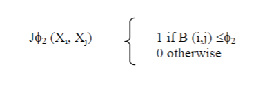 |
| For a given biological difference matrix (B) with values within the [0, 1] interval, we tend to continue and form a desired biological answer, wherever φ a pair of may be a threshold within the [0, 1] interval. By applying to all or any pairs of objects from a given knowledge set (with a hard and fast threshold), we tend to acquire a desired biological answer, supported external info extracted from the GO |
| Step 6: Performance evaluation |
| Measures are evaluated relating to their strength to noise, considering data with totally different noise levels. IBSA is that the metric accustomedvaluate distances for the cluster of genes. ISA willsolely be computed for knowledge sets with a customary partition, i.e.,class labels. As class labels aretypicallyunavailable for genecluster (e.g., time-series data), information is provided by the Gene ontology(GO) to beat the absence of labelled data. For the given threshold, actuality Positives (TP), False Positives (FP), True Negatives (TN), and False Negatives (FN) area unit given by the subsequent |
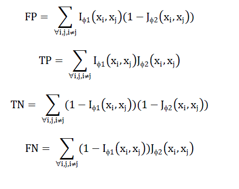 |
| Then False positive rate given by FPR=FP/(FP+TN) and True positive rate given by TPR=TP/(TP+FN) is computed and the AUC (area under curve) is plotted. AUC value of 1 indicates a distance that perfectly separates cancer samples according to the desired solution. An AUC value closer to or smaller than 0.5 labels a distance measure that fails to isolate objects according to desired solution. |
RESULTS AND DISCUSSION
|
| The results for both cancer data and time course experiments are presented. A total of 12 proximity measures are evaluated for 4 datasets (with and without noise) including a time-course dataset. Fig. |
| In the below fig 1.Shows the performance graph plotting the Area under curve values with the correlation and distance measures. The AUC Values will be between 0 and 1. Since the AUC value closer to one indicates the measure which best separates the cancer samples according to desired solution, the results show that the Minkowski distance measure is the best measure |
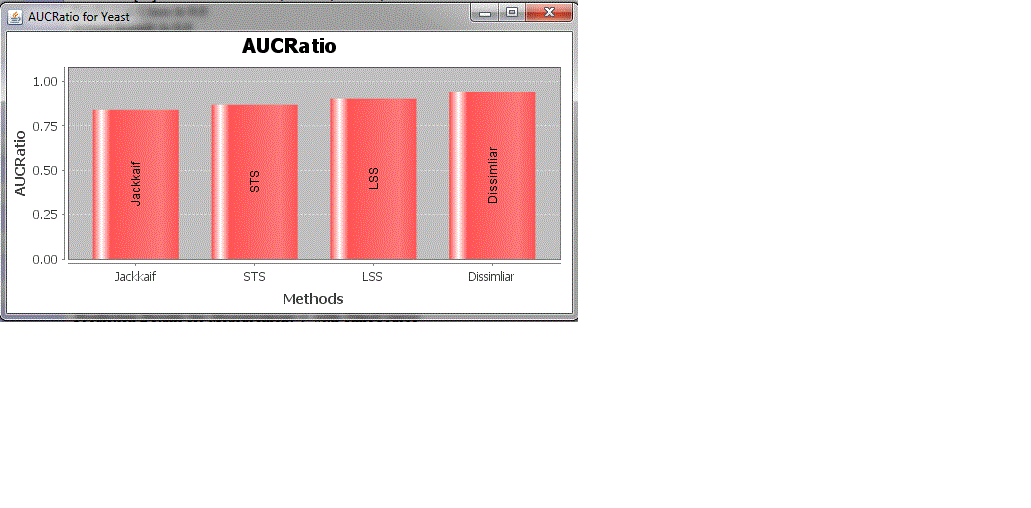
| The figure 2 indicates the performance of time-course specific measures and the four time course specific measures used here are Jack-knife, Short-time series dissimilarity, Local shape based similarity, Yr1and ys1 similarity. And the graph shows that the yr1 and ys1 dissimilarity as the best measure. |
| The above figures 5 and 6 indicates the AUC chart for time-course specific measures and other measures The results indicate the Minkowski distance measure as the best measure among the correlation and distance measures. Also the YR1 and YS1 dissimilarity measure is found as the best measure among the time course specific measures. |
CONCLUSION AND FUTURE WORK
|
| Given their variations, Proximity measures are evaluated one by one for cancer and time-course experiments. With the exception of the comparison of proximity measures, a collection of time-course benchmark informationat the side ofa brand new methodology (IBSA) are introduced to judge distances for the cluster of genes. IBSA will beutilizedto judge proximity measures concerning any geneclustering application, i.e., it's not restricted to gene time-course information. The cancer and time-course experiments possess quite completely differentcharacteristics, thatought to be taken into considerationoncechoosing a proximity measure. For these 2 application eventualities, 2completely different proximity measures stood out as promising alternatives, i.e., Minkowski for cancer information and YS1 for time-course experiments. |
| With the connotation of improve the performance and accuracy of the system, we tend to propose a completely unique approach for measure referred to as “Consensus function” as the future work. Based on this consensus functionwe are able to improve the accuracy and true positive rate of the cluster of Gene Expression Microarray Data. Here we tend touse the hybrid bipartite graph formulation (HBGF) as the consensus function. |
Figures at a glance
|
 |
 |
 |
 |
| Figure 1 |
Figure 2 |
Figure 3 |
Figure 4 |
|
References
|
- A.A. Alizadeh et al., “Distinct Types of Diffuse Large B-Cell Lymphoma Identified by Gene Expression Profiling.” Nature, vol. 403, no. 6769, pp. 503-511, 2000.
- A. Zhang, Advanced Analysis of Gene Expression Microarray Data, first ed. World Scientific, 2006.
- D. Jiang, C. Tang, and A. Zhang, “Cluster Analysis for Gene Expression Data: A Survey,” IEEE Trans. Knowledge Data Eng., vol. 16, no. 11, pp. 1370-1386, Nov. 2004.
- G. Kerr, H.J. Ruskin, M. Crane, and P. Doolan, “Techniques for Clustering Gene Expression Data,” Computers Biology Medicine, vol. 38, no. 3, pp. 283-293, 2008.
- L.J. Heyer, S. Kruglyak, and S. Yooseph, “Exploring Expression Data: Identification and Analysis of Coexpressed Genes,” Genome Research, vol. 9, no. 11, pp. 1106-1115, 1999.
- M.B. Eisen, P.T. Spellman, P.O. Brown, and D. Botstein, “Cluster Analysis and Display of Genome-Wide Expression Patterns,” Proc. Nat’l Academy Sciences USA, vol. 95, no. 25, pp. 14863-14868, 1998.
- P. D’haeseleer, “How Does Gene Expression Clustering Work?” Nature Biotechnology, vol. 23, no. 12, pp. 1499-1501, 2005.
- S. Ramaswamy, K.N. Ross, E.S. Lander, and T.R. Golub, “A Molecular Signature of Metastasis in Primary Solid Tumors,” Nature Genetics, vol. 33, no. 1, pp. 49-54, Jan. 2003.
- T.R. Golub et al., “Molecular Classification of Cancer: Class Discovery and Class Prediction by Gene Expression Monitoring,” Science, vol. 286, pp. 531-537, 1999.
|