Encho Leo Tanyam1*Okolo Abraham2
1Department of Mathematics and Computer Science, University of Bamenda, Bambili, Cameroon
2Department of Statistics and Operations Research, Modibbo Adama University of Technology, Yola, Nigeria
Received: 13-Feb-2024, Manuscript No. JSMS-24-127523; Editor assigned: 16-Feb-2024, Pre QC No. JSMS-24-127523 (PQ); Reviewed: 01-Mar-2024, QC No. JSMS-24-127523; Revised: 13-Apr-2025, Manuscript No. JSMS-24-127523 (R); Published: 20-Apr-2025, DOI: 10.4172/jsms.11.1.001
Citation: Tanyam EL, et al. Analysis of Inventory Coordination in Supply Chain with Price Dependentent in a Stochastic Demand. RRJ Pharm Anal.2025;11:001.
Copyright: © 2025 Tanyam EL, et al. This is an open-access article distributed under the terms of the Creative Commons Attribution License, which permits unrestricted use, distribution and reproduction in any medium, provided the original author and source are credited..
Visit for more related articles at Research & Reviews: Journal of Statistics and Mathematical Sciences
The maximization of profits in the supply chain involves the coordination of key processes in the firm such as order placement, order fulfillment and purchasing which are supported by marketing, finance, engineering, information systems, operations and logistics. This study is on the coordination of three level supply chain networks with a single manufacturer supplying a single product to a single supplier who also supplies a group of retailers in a single consolidated quantity. The objective is to determine the optimal inventory policies for the manufacturer, supplier and retailer that minimize total system cost while meeting customer demand. We focused on modelling and optimization of three level supply chain with price dependent demand for optimal replenishment quantity, inventory ratio and annual total relevant cost with and without coordination. A numerical illustration is carried to observe the behavioural pattern of the decision variables with positive integer. The parametric analysis is carried out to observe the variation in optimal values of the decision variables with respect to variation in manufacturer, supplier and retailer ordering costs and selling prices.
Supply chain; Coordination; Price dependent demand; Total relevant cost
Managing supply chains in today’s distributed manufacturing environment has become more complex. To remain competitive in today’s global marketplace, organizations must streamline their supply chains. The practice of coordinating the design, procurement, flow of goods, services, information and finances, from raw material flows to parts supplier to manufacturer to distributor to retailer and finally to consumer requires synchronized planning and execution.
However, retailers, suppliers and manufacturers often make decisions according to the maximization of their profits in the process of supply chain management and then there exists a variety of conflicts among supply chain and supply chain members, which influences the stability and sustainability of the supply chain [1]. The maximization of their profits in the process involves the coordination of key processes in the firm such as order placement, order fulfillment and purchasing which are supported by marketing, finance, engineering, information systems, operations and logistics.
Coordination refers to managing challenges due to interdependencies among business entities by aligning goals, processes/functions, decisions and activities. That is, the management of dependencies between activities to achieve collectively goals that individual actors cannot meet. If products are to be supplied to the market (consumers) efficiently and effectively, then coordination will enable the right products in the right quantities to be supplied at the right place, at the right moment at minimal cost. This enable business entity to align their fulfillment process and coordinate their decisions on capacity, inventory, pricing and promotion, quality of the product or service and product variety.
Our objective is to determine the optimal inventory policies for the manufacturer, supplier and retailer that minimize total system cost while meeting customer demand.
Some research studies in supply chain coordination include; Blumenfeld, et al., which analysed trade-offs between transportation, inventory and production set-up costs over an infinite time horizon in order to determine optimal shipping strategies (routes and shipment sizes) on freight networks [2]. Hossain, et al., formulated mixed integer linear fractional programming models that maximize the ratio of return on investment [3]. Their results show that by coordination, the individual profit over and above joint profit could be increased and consumers purchasing price could be decreased.
Zhi-yang, et al., studied a coordination problem of a supply chain consisting of two competitive suppliers and a dominant retailer [4]. His results revealed that the decision variables and overall profit of the supply chain of suppliers and retailers under centralized decisions are better than those under the decentralized decisions.
Chandra, et al., investigated the benefit of the coordination between production and distribution planning over a finite time horizon by comparing it with a case, in which production and distribution are controlled separately [5]. In addition, Thomas, et al., reviewed the coordination issues among functional stages of the supply chain, such as procurement, production and distribution stages, at an operational level [6]. Manoj, presented a systematic literature review to elaborate the term coordination and enlist the important coordination mechanisms. According to Tiantian and Yezhuang, supply chain coordination impacts the enterprise performance positively and indirect impacts the enterprise performance through quality, cost and flexibility.
Vijayender, et al., considered coordination in a supply chain with a manufacturer, a retailer and two different consumer segments. The manufacturer decides on the wholesale price and the selling price is determined by the retailer. Wang, et al., studies coordination problem under disruptions capturing by the change of market scale and price sensitive coefficient in a one-supplier-one-retailer supply chain system. Xiangwen, et al., investigated the coordination policies for products subject to midlife price declines during their short product life cycles. They examined a two-period supply chain model consisting of one supplier and one retailer to identified policies and/or conditions under which the supply chain can be coordinated and a win-win situation can be guaranteed. Kang, et al., considered a two-level supply chain in which a supplier serves a group of retailers in a given geographical area to determine the replenishment time and quantity for each retailer by using the information on demands and inventory levels of the retailers to minimize total service cost (which is the sum of the fixed vehicle cost, retailer-dependent setup cost) and inventory holding cost of the whole supply chain [7].
Sundar, et al., considered two level supply chain networks with a single manufacturer supplying a single product to a single retailer to optimize the cost at each level and total relevant cost of the supply chain. Hematyar, et al., investigated an improvement in a win-win situation for members of supply chain consisting of one manufacturer and one retailer facing consumer return and stochastic demand that is sensitive to both sales effort and retail price. They revealed that demand is influenced by both retail price and retail sales effort. Hu et al., investigated a coordination mechanism for a supply chain with one manufacturer and one retailer in a single period, single product newsvendor model [8]. They concluded that if supply chain is coordinated its optimal actions (production quantity and warranty length) are realized while each party maximizes its own respective profit.
Huang, et al., studied the coordination problem of a supply chain comprising one supplier and one retailer under market demand disruption [9]. They adopted a novel exponential demand function and the introduced penalty cost to explicitly capture the deviation production cost caused by the market demand disruption. Their aim was to obtain the optimal strategies for different disruption scale under the centralized mode and to prove that for the decentralized mode, the supply chain can be fully coordinated by adjusting the price discount policy appropriately when disruption occurs. Han, et al., addressed a two-level supply chain consisting of multiple suppliers and a manufacturing plant with the objective to minimize total costs associated with the supply chain.
For levels inventory coordination, Lee, et al., developed inventory models for the three level supply chain (one supplier, one warehouse and one retailer) to determine the optimal integer multiple at n time interval to minimize the coordinated total relevant cost. Arshinder, et al., explored the applicability of coordination elements through an analytical model in three-level (Manufacturer–distributor–retailer) serial supply chains using contracts to improve certain performance measure beforehand [10].
Bo Yan, et al., used the profit distribution model based on the improved revenue sharing contract to coordinate a three-level supply chain in Fresh Agricultural Product (FAP) that comprises a manufacturer, distributor and retailer in Internet of Things (IoT) to improve the revenue-sharing contract and to determine the optimal solution when the supply chain achieves maximum profit in three types of decision-making situations. They concluded that there is benefit in revenue-sharing contract to all entities in the supply chain. Giri, et al., obtained an optimal order quantities and expected profits of the individual channel in a three-layer supply chain with one raw material supplier, one manufacturer and one retailer [11]. They also examined the effects of both supply chain coordination as well as sub-supply chain coordination for the centralized system and decentralized system under commonly used price-only contract. They also used a semi-integrated models under-price only contract to compare the optimal strategies under different power structures and the effects of the channel parameters on the optimal strategies. They concluded that there was a growing decentralization among the involved entities and hence minimizing the double marginalization effect inside the chain, especially when the end-customers' demand was not deterministic.
Md. Tariqul, et al., (2020) developed an inventory model that addresses the problem of a manufacturer having an imperfect production system with single supplier and single retailer and considers the Quantity of product (Q), Reorder points (r) and reliability factors (n) as the decision variables. They considered that the supplier may not be able to deliver the exact amount all the time a manufacturer needed and the demand and the time interval between successive availability and unavailability of supplier and retailer follow a probability distribution. They used a genetic algorithm to find the optimal solution and compare the results with those obtained from simulated annealing algorithm. Their Findings revealed that the optimal value of the decision variables to maximize the average profit in each cycle.
In our study we considered a three level coordination of inventory from the manufacturer to the supplier and from the supplier to the customers through a consolidation center in a distribution network. That is, stock from the supplier have one release time and are consolidated into a single shipment to the consolidation center at the supplier side.
In this section, we used the Economic Order Quantity (EOQ) model to develop a mathematical model in a coordinated three level supply chain network with price dependent demand for single manufacturer supplying a single product to a supplier who supplies to a group of retailers at market regions. The objective is to identify minimum optimal policies of inventory decisions for improvement of the supply chain (Figure 1).

Figure 1. The structure of supply system.
The retailers initiate the ordered quantity, qR, of the product from the supplier who then ordered an integer multiple of the retailers ordered quantity, qR, from the manufacturer. That is qM=qV=nqR, where qM is the manufacturer produced quantity, qV (where qV=nqR) is the suppliers ordering quantity in units, qR, is the retailers ordered quantity in units and n the number of ordered quantity by the retailer through the supplier. When the manufacturer supplies the ordered quantity, qV, to the supplier, he then shipped the quantity, qR, to the retailers. We assumed that there are no other suppliers for this product and the company is the sole manufacturer.
To derive the total cost of the supply chain we modelled the total variable costs of the component at each of their point of view.
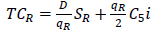
a) The total variable costs of the retailer point of view.
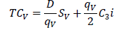
b) The total variable costs of the supplier point of view.
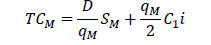
c) The total variable costs of the manufacturer point of view.
We modelled an optimization of three level supply chain with price dependent demand for optimal replenishment quantity, inventory ratio and annual total relevant cost with and without coordination.
Mathematical model
In order to keep the model mathematically tractable, we consider a simplified framework based on Sundar, et al., of two level supply chain with a single manufacturer supplying a single product to a single retailer to three level supply chain network with a single manufacturer supplying a single product to a supplier who is serving a group of retailers that serve multiples customers at a market region. Let first define the following notations:
SM: Manufactures ordering cost
hM: Manufacturers carrying cost
C1: Manufacturers manufacturing cost
C2: Manufacturers selling price in FCFA/unit
SV: Suppliers ordering cost
hV: Suppliers carrying cost
C3: Suppliers purchase price
C4: Suppliers selling price
SR: Retailers ordering cost
hR: Retailers carrying cost
C5: Retailers purchase price
C6: Retailers selling price
i: Interest rate
D: Annual demand in units
qR: Retailers ordering quantity in units
qV: Suppliers ordering quantity in units
qM: Manufacturers ordering quantity in units
n: The ratio of the manufacturer’s ordering quantity to suppliers to retailers ordering quantity, a positive integer
TC: Total annual cost of the supply chain
Assumptions of the model
The mathematical models in this article are developed based on the following assumptions.
1) The supplier is also a dealer of the same product.
2) Demand is a function of price.
3) Manufacturer’s inventory is some multiple integer of supplier’s inventory.
4) Supplier’s inventory is some multiple integer of retailer’s inventory.
5) Lead time is constant and known, that is, replenishment is instantaneous.
6) Shortages are not allowed. That is, there are always enough inventories on hand to meet the demand.
We also assumed that decisions are made on the basis of price; one can make use of the Economic Order Quantity (EOQ) to obtain an optimal solution for our problem.
In our model we considered profit among the components since Demand is price dependent and the final customer demand for the product (denoted by D) depends linearly on the price ρ per unit set by each component, i.e.,
D=a-bρ (1)
Where a and b are constants with a,b>0 and p is a selling price equal to C4 and C6 respectively. Each unit of item costs ρ francs. Backorders are not allowed since the retailers have to order enough to satisfy all the demand.
The total variable costs of the component at each of their point of view are obtained. According to Sharma (2007), suppose at the beginning of the inventory cycle time the maximum amount of inventory equal to the order quantity Q.
Let the level of inventory demanded be denoted by D. During a reorder cycle the quantity q is received and consumed. The graphical solution of this inventory is shown in Figure 2.

Figure 2. Inventory model with constant demand and instantaneous supply.
Suppose each time a fixed quantity q is ordered, the number of times the annual demand will be shipped will be D/q, where D is the total demand.
Annual carrying cost=Average inventory level × Carrying cost/unit/yea
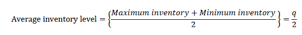
Carrying cost per unit per year = Retailerpurchase × Interest=Cki. (where k=C1C3 and C5 respectively).
Therefore,
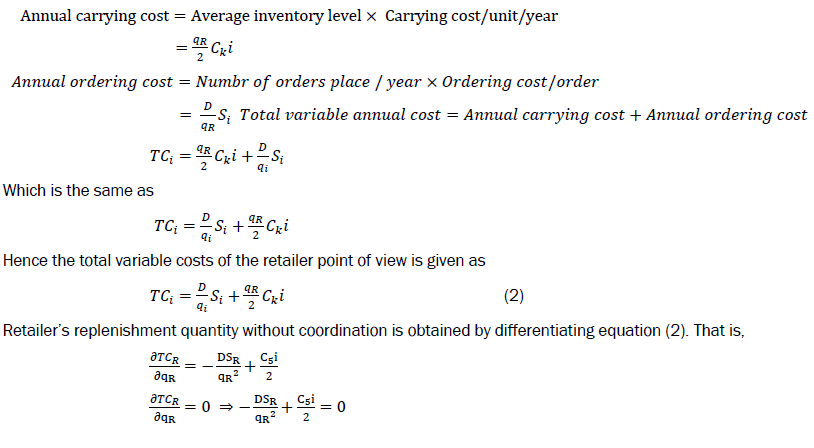
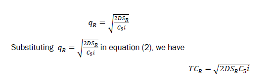
This is the corresponding optimal cost of the retailer without coordination.
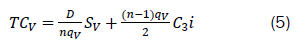
The total variable costs of the supplier point of view is given as
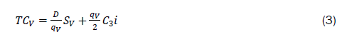
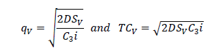
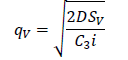
In a similar manner, the supplier’s replenishment quantity and the corresponding optimal cost without coordination is
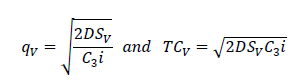
In a similar manner, the supplier’s replenishment quantity and the corresponding optimal cost without coordination is
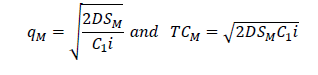
The total variable costs of the manufacturer’s point of view may be given as
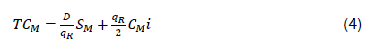
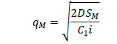
Also, the manufacturer’s replenishment quantity and the corresponding optimal cost without coordination is
| Manufacturer point of view | Supplier point of view | Retailer point of view |
 |
 |
 |
 |
 |
 |
 |
 |
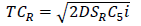 |
Table 1. Summary of independent decision variables without coordination
It is assumed that supplier’s inventory is multiple of retailers ordering quantity and it can be written as

The total variable costs of the supplier point of view may be given as
Total cost of the supply chain is given by
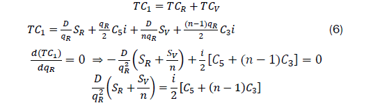
By Sundar, et al., the optimal, retailer’s quantity is given as,
By substituting the optimum values of replenishment quantity in equation (6) the total cost of the supply chain is obtained.
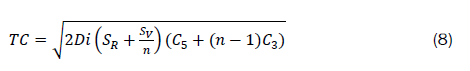
To find the integer value of this maximizes the Total Cost (TC),
Thus, the total variable cost at the manufacturer from supplier is given by

Also, it is assumed that manufacturer’s and supplier’s inventory is multiple of retailers ordering quantity and it can be written as qM=qV=nqR.
The total cost of the supply chain is given by
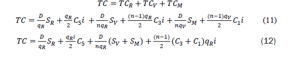
Our objective is to find the retailer’s optimum value of quantity, qR, to minimize the average total cost with coordination, i.e,. we differentiate equation (12) with respect to qR to obtain
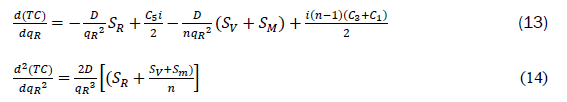
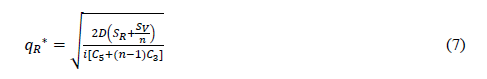
Equating (d(TC))/(dqR)=0 in equation (13) and solving for qR we have
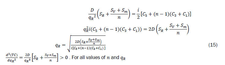
Hence n and qR become optimum
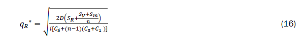
qR*is retailer’s optimum value of quantity, q, that will minimize the average total cost with coordination. The corresponding optimal cost of the supply chain is obtained by substituting the optimum values of replenishment quantity of equation (16) in equation (12). That is
By simplifying the above equation gives
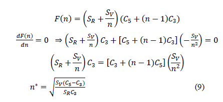
We can find the integer value of n that maximizes equation (16).
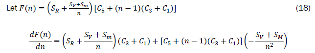
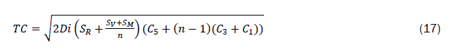
For the integer value of n that maximizes equation (14), dF(n)/dn=0 . Thus,
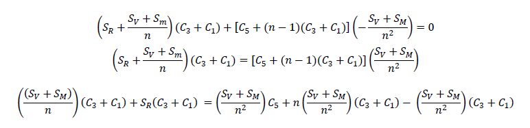
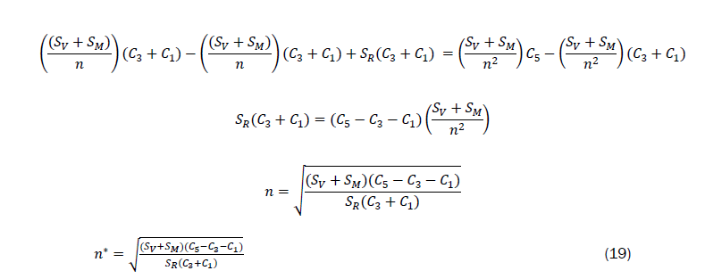
In general this will not be an integer.
Hence we find F(n1), F(n2) and F(n3)) where n1, n2 and n3 are integers surrounding the n*.
If F(n1) ≤ F(n2)→n=n1and if F(n1) ≥ F(n2)→n2
Similarly, if F(n2) ≤ F(n3) →n=n2 and if F(n2) ≥ F(n3)→n=n3
Also, we obtain the minimum optimal total relevant cost of the supply chain by substituting the value of n* in equation (17).
Numerical illustration
We considered an item with the following variables and constant values, the equations are solved using Microsoft Office Excel 2007. We used the data in Table 2 and obtained an approximate value of a=10000 and b=0.7.
|
S/N |
Months (Source) |
Demand (Units) |
Unit cost |
Cost (F CFA) |
|
1 |
July |
206000 |
14 |
2884000 |
|
2 |
August |
143000 |
14 |
2002000 |
|
3 |
September |
234000 |
14 |
3276000 |
|
4 |
October |
286000 |
14 |
4004000 |
|
5 |
November |
181000 |
14 |
2534000 |
|
6 |
December |
220000 |
14 |
3080000 |
|
7 |
January |
204000 |
14 |
2856000 |
|
8 |
February |
204000 |
14 |
2856000 |
|
9 |
March |
204000 |
14 |
2856000 |
|
10 |
April |
280000 |
14 |
3920000 |
|
11 |
May |
188000 |
14 |
2632000 |
|
12 |
June |
129000 |
14 |
1806000 |
|
13 |
July |
213000 |
14 |
2982000 |
|
14 |
August |
35000 |
14 |
490000 |
|
15 |
September |
108000 |
14.2 |
1535760 |
|
16 |
October |
86000 |
14.2 |
1222920 |
|
17 |
November |
131000 |
14.2 |
1862820 |
|
18 |
December |
26000 |
14.2 |
369720 |
|
Total |
3078000 |
37457220 F CFA |
Table 2. Production capacity (in cases).
The data in Table 2 represent the production capacities and expected demands for one of its product, which is small stout guinness from July 2011 to June 2012. The company brews and packages the small stout guinness into bottles. The bottle contains 300 ml of Small Stout Guinness and is packaged in cases. A case contains 24 bottles, each with total volume of 0.072 hectolitres.
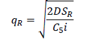
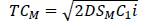
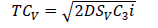
The second column deals with months within which the data were collected, thus from July 2011 to December 2012. The third column describes the demand amount that must be produced to meet the request made by their client. The highest demand was recorded in the month of April, 2012. The lowest demand was recorded in the month of December, 2012. The total demands were 3078000. The fourth column describes the unit cost. The fifth column describes the cost amount that must be sold for the given production demand and the total cost was 37457220 F CFA By using the value of a=1000, b=0.7, SM=220900 per order, SV=4700 per order, SR=1000 per order, C1=150, C2=225,C3=225,C4=400, C5=400, C6=500 and i=0.15 (15%) the optimal values of the decision variables without coordination are as follows. We substituted C6=500 in equation (1) to obtain the total demand of the retailers D=9650. Substituting the values of SR, C5, i and D=9650 in qR=√((2DSR)/(C5 i)) and TCR=√(2DSR C5i) the retailer’s replenishment quantity qR=804.98 units and the total cost at retailer’s point, TCR=48124.84 are obtained. Similarly, substituting C4=400 and C2=225 in equation (1) the value of the total demand of the suppliers and manufacturers are given as 9895 and 9842.5, respectively. Substituting SV, C3, i, supplier’s demand D=9895 in qV=√((2DSV)/(C3i)) and SM, C1, i, manufacturer’s demand D=9842.5 in qM=√((2DSM)/(C1i)) their respective replenishment quantities are 2916.32 units and 4396.17 units given their total costs at their various points of view as 55530.8 from TCV=√(2DSVC3i) and 98913.79 from TCM=√(2DSMC1i). The minimum total cost of the supply chain (TC) without coordination is the sum of TCR, TCV and TCM which gives TC=202569.43.
The optimal values of the decision variables with coordination are obtained as follows; the value of the inventory ratio is obtained by substituting the values of SR, SV, SM, C1, C3 and C5 in equation (19) to get n=2 and the corresponding retailer’s replenishment quantity qR (opt) is obtained by substituting the retailer’s total demand D=9650, SR=1000, SV=4700, SM=22090 and n=2 in equation (16) to get 1545.92 units. Substituting this value of qR (opt) and the values of i, SR and C5 in equation (2), the minimum total cost at retailer point of view is obtained as TC=52810.43. Since qM=qV=nqR, the supplier’s and the manufacturer’s replenishment quantities are, qV=3091.84 and qM=3091.84, respectively. The minimum total cost at the supplier’s points of view is obtained from equation (5) to give TCV=46298.69 while the minimum total cost at the manufacturer’s point of view is obtained from equation (10) to obtain, TCM=51909.67 with the minimum total supply chain from equation (17) given as, TC=179713.60.
Upon salvation of the equations, the optimal values of the variables with and without coordination are summarized in Table 3.
| S/N | Parameters | Without coordination | With coordination |
| 1 | Inventory ratio, n | 3 | 2 |
| 2 | Retailer’s replenishment quantity, qR | 804.98 | 1545.92 |
| 3 | Supplier’s replenishment quantity, qV | 2934.64 | 3091.48 |
| 4 | Manufacturer’s replenishment quantity, qM | 4407.88 | 3091.48 |
| 5 | Total cost at retailer’s point, TCR | 48299.07 | 46298.69 |
| 6 | Total cost at supplier’s point, TCV | 55879.63 | 52053.24 |
| 7 | Total cost at Manufacturer’s point, TCM | 99177.24 | 51909.67 |
| 8 | Total cost of the supply chain, TC | 203355.9 | 179713.6 |
Table 3. Supply chain parameters without and with coordination.
The increase in the total variable inventory cost due to increase in the order quantity is expressed as in (Sharma, 2007):

Let the ordered size without coordination (TVCwithout) be k times the ordered size with coordination (TVCwithout) (EOQ). i.e., TVCwithout=k(TVCwith)
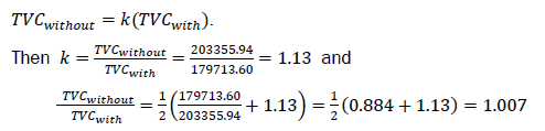
This implies that, if order quantity is increased by 13%, the total cost would increase by 0.7 percent. There is also a reduction of 12% of the total cost inventory without coordination to inventory with coordination.
A comparison of replenishment quantity at retailer’s level, supplier’s level and manufacturer’s level with coordination and without coordination are represented in Figure 3.

Figure 3. Comparison of replenishment quantity at retailer’s level, supplier’s level and manufacturer’s level with coordination and without coordination.
From Figure 3, it is clearly indicative that replenishment quantity at the retailer is more without coordination rather than with coordination. The replenishment quantity at the supplier is more with coordination rather than without coordination whereas the manufacturer’s replenishment quantity with coordination is less rather than without coordination. It is due to the fact that with supply chain coordination the number orders at the retailer is less rather without coordination.
A comparison of minimum cost at retailer’s level, supplier’s level, manufacturer’s level and the total supply chain with coordination and without coordination are represented in Figure 4.

Figure 4. Comparison of total cost at retailer’s level, supplier’s level and manufacturer’s level with coordination and without coordination.
From Figure 4, it is observed that retailer’s cost with coordination is more rather than without coordination. The supplier’s cost with coordination is less rather than without coordination whereas manufacturer’s cost with coordination is less rather than without coordination. However, the total relevant cost of the supply chain with coordination is less rather than without coordination. It is attributed to the fact that the rate of increase in carrying cost is less than the rate of decrease in ordering costs. The above results followed the same pattern.
The optimal values of the decision variables of three level supply chain with coordination are obtained as follows; the value of the inventory ratio is obtained by substituting the values of SR, SV, SM, C1, C3 and C5 in equation (23) to get n=2 and the corresponding retailer’s replenishment quantity qR (opt) is obtained by substituting the retailer’s total demand D=9650, SR=1000, SV=4700, SM=22090 and n=2 in equation (20) to get 1545.92 units. Substituting this value of qR (opt) and the values of i, SR and C5 in equation (2), the minimum total cost at retailer point of view is obtained as TC=52810.43 . Since qM=qV=nqR, the supplier’s and the manufacturer’s replenishment quantities are, qV=3091.84 and qM=3091.84, respectively. The minimum total cost at the supplier’s points of view is obtained from equation (5) to give TCV=46298.69 while the minimum total cost at the manufacturer’s point of view is obtained from equation (10) to obtain, TCM=51909.67 with the minimum total supply chain from equation (21) given as, TC=179713.60. Table 4 shows the calculated results of the optimal replenishment quantities of the retailer, supplier, manufacturer and the optimal minimum costs of the retailer, supplier, manufacturer and total supply chain when the value of n is varied.
| N | qR | qV | qM | TCR | TCV | TCM | TC |
| 1 | 2549.74 | 2549.74 | 2549.74 | 76430.69 | 42893.01 | 42734.85 | 179390.1 |
| 2 | 1545.92 | 3091.84 | 3091.84 | 46298.59 | 52053.24 | 51909.62 | 179713.6 |
| 3 | 1130.34 | 3391.02 | 3391.02 | 33817.8 | 57107.39 | 56970.25 | 181822.6 |
| 4 | 899.17 | 3596.68 | 3596.68 | 26871.5 | 60581.27 | 60448.11 | 184346.1 |
| 5 | 751.12 | 3755.6 | 3755.6 | 22420.25 | 63265.46 | 63135.14 | 187008.5 |
| 6 | 647.92 | 3887.52 | 3887.52 | 19315.56 | 65493.5 | 65365.41 | 189718.7 |
| 7 | 571.74 | 4002.18 | 4002.18 | 17022.28 | 67429.95 | 67303.71 | 192438.6 |
| 8 | 513.14 | 4105.12 | 4105.12 | 15257.07 | 69168.41 | 69043.76 | 195150.3 |
| 9 | 466.61 | 4199.49 | 4199.49 | 13854.49 | 70762.09 | 70638.86 | 197844.2 |
| 10 | 428.76 | 4287.6 | 4287.6 | 12712.78 | 72250.03 | 72128.06 | 200515.4 |
Table 5. Optimal values of the decision variables and objective function with respect to inventory ratio (n) in three level supply chain.
As in Table 4 of two level supply chain by Sundar, et al. Table 5 of three level supply chain shows a similar pattern. That is, the replenishment quantity of the retailer is decreasing whereas that of the supplier and manufacturer increases with increase in positive inventory ratio, (n). The total cost of retailer decreases with increased inventory ratio whereas the supplier, manufacturer and supply chain increases with the corresponding increase in the inventory ratio, (n). The percentage change in the minimum optimal total relevant cost from two level supply chain to three level supply chain is 36% with an increase of 50% optimal inventory replenishment quantity. The values in Table 5 can also be represented graphically.
In Table 5 and Figure 5, it is observed that the retailer replenishment quantity reduces as the inventory ratio (n) increases. The supplier’s and manufacturer’s replenishment quantities are increasing as the inventory ratio (n) increases. This is due to the fact that retailer’s inventory level varies inversely with an increase in inventory ratio (n) whereas supplier’s and manufacturer’s inventory varies proportionally with an increase in inventory ratio (n).

Figure 5. Variation of retailer’s, supplier’ and manufacturer’s ordering quantity with positive integer.
In Table 5 and Figure 6 shows the analysis of variation of total cost at retailer’s point, supplier’s point, manufacturer’s point and supply chain with inventory ratio (n). From this Table 5 or Figure 6, it is analysed that the total relevant cost of the supply chain (TC) initially reduces and becomes optimum, then increases gradually as the inventory ratio increases. The total relevant cost at the manufacturer’s and supplier’s points increases gradually whereas at retailer’s point decreases with an increase in inventory ratio. According to Sundar, et al., it is attributed to the fact that the proportionate decrease in carrying cost is less than the proportionate increase in ordering cost at retailer’s point where as the proportionate decrease in the set up cost is less than the proportionate increase in carrying cost. Consequently total cost of the supply chain increases [12].

Figure 6. Variation of total cost at retailer’s point, supplier’s point and Manufacturer’s point and supply chain with inventory ratio (n).
Table 6 and Figure 7 show the analysis of variation of retailer’s replenishment quantity at retailers point with positive inventory ratio for particular values of retailers selling price. The curve shows that the retailer replenishment quantity gradually decreases with increase in positive inventory ratio. It is due to the fact that the size of order increases while the ordering cost decreases whereas the inventory carrying cost increases. Consequently retailers prefer to maintain less inventory level. Inventory is shipped from supplier to retailers through less number of shipments.
Also it is observed from Figure 7, that there is no appreciable change in trend pattern of retailer’s replenishment quantity though there is a change in retailers selling price [13-15]. This is attributed to the fact that the change in retailer’s selling price has no significant impact on optimal values of decision variables.
| C6 | 500 | 550 | 600 | |
| S/N | qR | TC | TC | TC |
| 1 | 2549.74 | 179390.1 | 179064.5 | 178738.3 |
| 2 | 1545.92 | 179713.6 | 179387.4 | 179060.6 |
| 3 | 1130.34 | 181822.6 | 181492.6 | 181161.9 |
| 4 | 899.17 | 184346.1 | 184011.5 | 183676.3 |
| 5 | 751.12 | 187008.5 | 186669.1 | 186329 |
| 6 | 647.92 | 189718.7 | 189374.3 | 189029.3 |
| 7 | 571.74 | 192438.6 | 192089.3 | 191739.4 |
| 8 | 513.14 | 195150.3 | 194796.1 | 194441.2 |
| 9 | 466.61 | 197844.2 | 197485.1 | 197125.3 |
| 10 | 428.76 | 200515.4 | 200151.4 | 199786.8 |
Table 6. Variation of Retailer’s replenishment quantity and total cost of the supply chain with positive inventory Ratio (n) and retailers selling price C6.
Figure 7 shows the analysis of variation of total relevant cost of the supply chain with positive inventory ratio for particular values of retailers selling price [16,17]. From this figure, the total cost of the supply chain remain the same no matter the retailers selling price as the inventory ratio increases from 1 to 2 whereas the total cost of the supply chain increases no matter the retailers selling price with an increase in inventory ratio above 2. Also from the figure, it is analysed that there is no appreciable change in trend pattern of total relevant cost of the supply chain though there is a change in retailers selling price. It is attributed to the fact that the change in retailer’s selling price has no significant impact on optimal values of decision variables [18-20].

Figure 7. Variation of total cost of supply chain, TC with positive inventory ratio (n) and retailers selling price (C6).
In this study, mainly, a mathematical model is developed for three level supply chain for coordination considering single manufacturer supplying a single product to a single retailer under-price dependent demand. The optimal values of the decision variables are determined with and without coordination. Based on the findings of this research, it is concluded that total relevant cost of the supply chain becomes less with coordination rather than without coordination. Average inventory level at the retailer becomes more whereas inventory level at the manufacturer becomes less.
In addition, the parametric analysis is carried to observe the variation in optimal values of decision variables and objective function. From these findings it is concluded that there is a significant impact of manufacturer’s unit cost on optimal values of the decision variables where as there is no appreciable variation in the trend pattern of decision variables with retailers selling price. Also, it is concluded that the variation in retailer’s ordering cost and manufacturer’s set up cost causes significant change in optimal values of the decision variables and objective function.
[Crossref] [Google Scholar] [PubMed]
[Google Scholar] [PubMed]