Automatic Brain Tumor Detection Using
K-Means and RFLICM

Dr. A.J.Patil; Dr.Prerana Jain; Ashwini Pachp; e

Automatic Brain Tumor Detection Using K-Means and RFLICM

Dr. A.J.Patil¹, Dr.Prerana Jain², Ashwini Pachpande³

Principal, Dept of Electronics and Telecommunication, S.G.D.C.O.E, Jalgaon, India¹
Professor, Dept of Electronics and Telecommunication, S.G.D.C.O.E, Jalgaon, India²
M.E Student, Dept of Electronics and Telecommunication, S.G.D.C.O.E, Jalgaon, India³

Related article at Pubmed, Scholar Google

Visit for more related articles at International Journal of Advanced Research in Electrical, Electronics and Instrumentation Engineering

Abstract

In this paper presented a simple method for detection of area of tumor in brain MRI. The tumor is an uncontrolled growth of tissues in any part of the body. As it is known, the brain tumor is inherently serious and life threatening. Most of research in developed countries shows that the numbers of people who have brain tumors were died due to the fact of inaccurate detection. Tumors have different characteristics and different treatment. However the manual tumor detection method of detection takes more time for the determination size of tumor. To avoid that, in this paper presented computer aided method for detection of brain tumor based on the combination of two algorithms, Kmeans and improved fuzzy C-means (RFLICM) algorithm for image segmentation by introducing weighted fuzzy factor local similarity measure to make a trade-off between image detail and noise. This method allows the segmentation of tumor tissue with accuracy. In addition, it also reduces the time for analysis. At the end of the process the tumor is extracted from the MR image and its position and the shape is determined.

Keywords

Segmentation, USM, K-Means, RFLICM, Canny edge detection, SCM classifier

INTRODUCTION

Nowa day?ssegmentation of medical images is very important as the images are large in number for diagnosis by radiologist. Image segmentation method is utilized to find objects and boundaries in an image. It is an important tool in medical image processing [1,2,3]. A segmentation of the brain structure from magnetic resonance imaging (MRI) has received much importance in recent times as MRI distinguishes itself from other modalities.MRI has as additional advantage as it can be applied in the analysis of brain tissues. Segmentation technology has greatly increased knowledge of normal and diseased anatomy for medical research and is a vital component in diagnosis and treatment planning. The objective of division is to improve and change the representation of a picture into something that is more genuine and easier for analysis. The basic attribute for segmentation are edges and texture. The result of segmentation method gives a set of regions that altogether cover the whole image which are extracted from the image. There are many conventional methods of MRI segmentation such as seed based region growing, partial differential equation (PDE) level set segmentation, graph based segmentation, split and merge based segmentation, edge based segmentation, clustering based segmentation. The problem with all these methods is that they need human interaction for accurate and authentic segmentation.

RELATED WORK

Exhaustive work has been done by several researchers in the area of image segmentation.Zaldeh (1965) introduced fuzzy set theory to clustering concept so it is named as fuzzy clustering. Matthew C. Clark et. al (1998) [4], proposed artificial intelligence techniques based on automated segmentation method using FCM and multispectral tool. Using a multi-layer Markov random field framework, Gering, et. al (2002) [5] proposed a method that identifies deviations from normal brains. M.N. Ahmed et. al (2002) [6], proposed a automatic segmentation technique using a new biascorrected FCM (BCFCM) algorithm for adaptive segmentation and intensity correction of MRI. Liang Liao et. al(2007) [7], proposed a method using more robust kernelized algorithm by joining Gibbs spatial constraints for the fuzzy segmentation of MRI data. J. J. Corso, et. al (2008) [8], proposed method used multichannel MRI volumes to detect and segment brain tumor. Fuzzy clustering is a very famous technique for detecting brain tumor. It has demonstrated the fuzzy clustering approach which provides better results for multi sequence data. Nikhil R. Pal et. al proposed the fuzzy-possibilistic c-means (FPCM) (2005) [9] algorithm. Hathaway and Hu, (2009) [10] have been proposed a new technique to improve the performance of standard FCM algorithm and to reduce its computational complexity. S.R. Kannanaet. al (2012) [11], proposed a robust FCM algorithms with kernel functions for segmentation of brain and breast medical images. Vida HaratiRasoulKhayatiet. al (2011) [12], proposed a fully automatic method for tumor region detection in brain MRI. Cai. Et Al. proposed the fast generalized FCM (FGFCM) algorithm, which can significantly reduce the execution time by clustering on the gray-level histogram rather than on pixels. It is less sensitive to noise to some extent because of the introduction of local spatial information. Maoguo Gong et. al (2012) [14] proposed reformulated fuzzy local information C-means clustering algorithm (RFLICM) segmentation technique.

WORK METHODOLOGY

The implemented system has mainly five modules asimage acquisition, image enhancement, segmentation of image using K-means algorithm, segmentation of image using RFLICM algorithm, feature extraction. The implemented method is a combinationof K- means and RFLICM algorithms. In the literature survey found that the conventional FCM algorithm is noise sensitive and complex [13,14]. In order to compensate this Maoguo Gong et. al [14] introduced RFLICM algorithm with weighted fuzzy factor local similarity measure. This method makes a tradeoff between image detail and noise. Fig. 1 shows system block diagram of implemented method.

A. Implemented System’s Block Digram

B. Image acquisition

MRI brain images for processing are obtained from internet database having featureT1-weighted (T1W), T2-weighted (T2W) and T2 Flair. The images contain soft brain tissues such as WM, GM and CSF are surrounded by bone structure. The WM, GM and CSF of the brain are represented by white, gray and black colors respectively except the background black color. These images are available in joint photo graphic (.jpg) format.

C. Image Enhancement

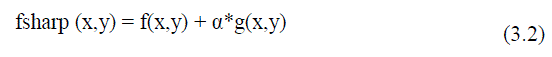
The enhancement method consists of two steps as median filter to reduce noise and unsharp mask (USM) filter for edge sharpening. This technique is applied to input data in order to remove noise and to sharpen edges.It?s necessary in order to assure that image satisfies certain assumptions for good segmentation according to Haralick and Shapiro [3]. Filtering can be utilized to take out undesirable components of noise.Median filtering is a prevalent technique of the image enhancement to remove salt and pepper noise without effectively reducing the image sharpness. Here, the median procedure was performed by sliding a 3x3 windowing operator over the image. Next step is USM is a classical tool for sharpening image [16, 17,18]. It is process that enhances edges and other high frequency parts in images. The USM improve the visual quality of images by emphasizing their high frequency portions that contain fine details. The two steps of unsharp mask filter [16] are mentioned equation(3.1) and (3.2) unsharp mask filter makes edges image g (x, y) from input images f (x, y).

Where, f smooth (x, y) is a smoothed form of f (x, y) (gaussian blur algorithm) the edge images from the result of subtracting input images from low pass signal could be utilized for image sharpening by adding it into the input signal.

Where, α is a scaling constant range 0-1.When α >1, the process is referred to as high boost filtering.The essential point of interest of the unsharp filtering over other sharpening filters is the control flexibleness on the grounds that a larger part of other sharpening filters does not supply any user-adjustable parameters.

D. K-means Segmentation method

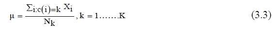
K-means clustering applied to output images of USM technique. K-means clustering [13] is the unsupervised learning algorithm. Clustering the image is gathering the pixels as per some attributes. In the K-means algorithm first need the number of clusters k. Then centers of k-cluster are chosen randomly. The distance between each pixel to each cluster center is calculated. The distance may be about simple Euclidean function. A single pixel is compared to all cluster centers utilizing the separation equation. The pixel is moved to specific cluster, which has the shortest distance among all. At that point the centroid is re-estimated again each pixel is compared to all centroids. The methodology proceeds until the center converges. Segmentation task is performed using orthonormal operators. Images having the tumor are processed using K-means clustering and significant accuracy rate of 75% is obtained [19]. The K-means algorithm divided into eight steps as follows:

1) Give the number of cluster values as the k.

2) Centers of the k - cluster are chosen randomly (μ).

3) Calculate mean or center of each cluster (μu (i)) given in (3.3).

4) If the distance is near, the center (μ==old μ) then moving to that cluster.

5) Calculate the distance between each pixel and each cluster center given in (3.4).

6) Otherwise, move to the next cluster.

7) Re-estimate the center.

8) Repeat the above process until the center does not move.

Mathematical representation to compute the cluster means μ

Calculate the distance between the cluster centers to each pixel

Where, N_k = Number of clusters, x_i = Data measured in d-dimensional, M_k = Cluster centers.

E. Segmentation Using Improved Fuzzy C-Means

Improved FCM applied to the final segment image of K-means segmentation. Clustering procedures fabricate a panel of data into clusters with similar entities grouped in a cluster and dissimilar entities in different clusters. In clustering process, the dissimilarity between any two elements of the dataset can be computed using distance measures. The fuzzy logic is a way preparing the information by giving the partial membership value to each pixel in the image. The membership value of the fuzzy set is ranging from 0 to 1. Among the clustering methods, the FCM algorithm is a standout amongst the most well-known routines since it can retain more data from the original image and has vigorous qualities for ambiguity. However, the traditional FCM algorithm is very sensitive to noise so it does not consider any information about the spatial context [15]. Recently, Krindis and Chatzis proposed a robust FLICM clustering algorithm to remedy the above shortcoming. The characteristic of FLICM is the use of a fuzzy local similarity measure which is aimed at guaranteeing noise insensitiveness and also the image detail preservation. A novel fuzzy factor is brought into the FLICM to improve the clustering execution [14]. The fuzzy factor can be defined mathematically as follows (3.5):

m = fuzzification factor (2),x_i= Image, C=represents the prototype value of the ith cluster ( V_k )

Where the ith pixel is the center of the local window, the jth pixel represent the neighboring pixels falling into the window around the ith pixel and dij is the spatial Euclidean distance between pixels i and j. Vk indicates the prototype of the center of cluster k, and Ukj indicates the fuzzy membership of the gray value j with respect to the kthcluster.It can be seen that factor Gki is defined without setting any artificial parameter that controls the trade-off between image noise and the image details. The impact of pixels within the local window Gki is applied adaptable by utilizing their spatial Euclidean separation from the central pixel. In this way, Gki reflect the damping extent neighbours with the spatial separations from the central pixel. By using the definition of Gki (3.6), the objective function of the FLICM defined in terms of

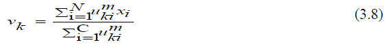
Where, Vk represents the prototype value of the kth cluster and Uki represents the fuzzy membership of the ith pixel with respect to cluster k, N is the number of the data items and C is the number of clusters 2 xi Vk is the Euclideandistance between object xi and the cluster centers Vk .In addition, the calculation of the membership partition matrix (3.7) and the cluster centers is performed as follows (3.8) [15]:

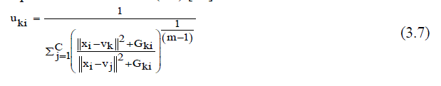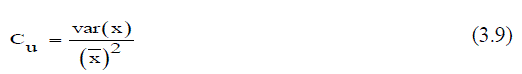
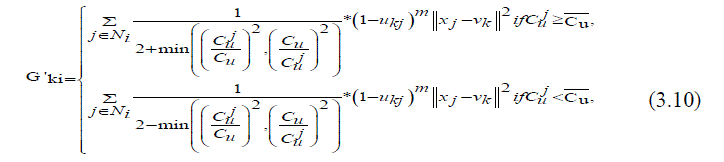
Modification on the FLICM is fuzzy factor Gki , it can be derived that the local gray level information and spatial information in Gki are represented by the gray level difference and spatial distance respectively. Krindis and Chatzis [14] endeavour to gauge the damping extent of the neighbours with the spatial separations from the central pixel. For the neighbourhood pixels with the same gray-level value, the greater the spatial distance is the smaller the damping extent and vice versa. However, the damping extent of the neighbours that is reflected by the spatial separations is just isolated into two categories (0.414) and neglects to comprehensively investigate the effect of each one neighbouring pixel onto the fuzzy factor Gki the foregoing analysis highlights the importance of the accurate estimation of the fuzzy factor Gki toeffectively suppress the influence of the noisy pixels. Keeping in mind at the end, goal is to remove defects mentioned above the local coefficient of variation is embraced to supplant the spatial separation. In addition, the local coefficient of variation Cu (3.9)[14,15] is defined by,

Where var(x) and X are the intensity variance and the mean in a local window of the image respectively. The value of Cu reflects the gray-value homogeneity degree of the local window. It displays high values at the edges or in the region tainted by noise and delivers low valuesin homogeneous areas. The damping extent of the neighbours with the local coefficient of variety is measured by the areal kind of the neighbour pixels located. In the event that the neighbour pixel and the central pixel are placed in the same area for example the homogeneous region or the area adulterated by noise, the results of the local coefficient of variation obtained from them will be very close and vice versa. Compared with the spatial distance the discrepancy of the local coefficient of variation between neighbouring pixels and the central pixel is relatively accordance with the graylevel difference between them. In addition, it helps to exploit more local context information since the local coefficient of variation of each pixel is computed in a local window. Here, the modified fuzzy factor G'ki (3.10)[18] can be defined as

Where Cu is the local coefficient of variation of the central pixel, j Cu represents the local coefficient of variation of neighbouring pixels, and Cu is the mean value of j Cu that is located in a local window. As shown in (3.10), the changed fuzzy factor G'ki adjusts the membership value of the central pixel considering the local coefficient and also the gray level of the neighbouring pixels. If there is a distinct difference between the results of the local coefficient of variation that are obtained by the neighbouring pixel and the central pixel, the weightings added of the neighbouring pixel G'ki It increased to suppress the influence of an outlier; thereby, the modified FLICM, i.e. termed as RFLICM, is expected to be more robust to its pre-existencefinally, by taking the place of G'ki In FLICM with the modified fuzzy factor G'ki .The RFLICM algorithm can be summarized as follows.

1) Set the values ofC,mand .

2) Randomly initialize the fuzzy partition matrix and set the loop counter b = 0.

3) Calculate the cluster prototypes using (3.8).

4) Compute the partition matrix using (3.7).

5) max U(b)U(b1) Then stop; otherwise set b = b + 1 and go to step (3).

F. Feature Extraction

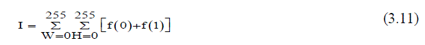
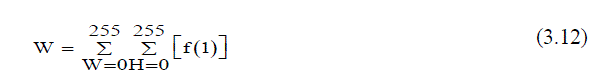
Area and perimeter are calculated fromsegmented tumor image. Area calculation is applied to output images of RFLICM. In this step tumor area on single slice calculated using the linearization method [6]. Image in binary form has only two values either black or white (0 or 1). For further operation here image resized to 256x256 size. The equation (3.11) shows that the binary image can be represented as a summation of total number of white and black pixels in the image,

Pixels =Width (W) X Height (H) = 256 x 256, f (1) = White pixel (digit 1), f (0) = Black pixel (digit 0). In order to calculate the area of tumor took the summation of the number of white pixels (digit 1) in binary image. Number of white pixels,

Where, W = number of white pixels.The area calculation formula is,

According to 96 dpi (dot per inch) 1 pixel = 0.264583333; Then 1/96 is the number of inches per pixel. There is 25.4 mili meters per inch, so 25.4 / 96 is the number of mili meter per pixel and that is the 0.264583333,approximate 1 Pixel = 0.264 mili meter.Perimeter calculation applied to output images of RFLICM. Tumor edge is extracted using the canny edge detection method. The canny edge detection algorithm implemented using a series of steps. First step is to smooth the image with a gaussian filter. Then computed the gradient magnitude and orientation using finitedifference approximations for the partial derivatives, after that a non-maxima suppression applied to the gradient magnitude. After this canny edge detection process obtained the perimeter of tumor image.

G. Lobe classification and stage classification

Lobe classification is applied to output image of RFLICM to find the position of tumor.Firstly obtained the centroid of tumor using MATLAB function „regionprops ()? which gives position of centroid with respective x-axis and with respective y-axis. Then the size of tumor calculated using MATLAB command „size ()? and columns of the image are divided into two equal partsand then compared with the x-axis position of the tumor. After the compassion it detects the tumour presence in right or left lobe.Stage classification applied to output images of RFLICM to find the stage of tumor classified on local based staging on a single slice. SVM has been used for tissue classification into two classes, namely stage 1 and stage 2. It is based on the concept of hyper plane that depicts choice limits. The principle motivation behind SVM is a change of information into higher measurement space in such a way where hyper plane divides with maximal separation from the closest preparing data [20].

RESULTS

The brain MRI slices of interest for the study described here could process axial and coronal slices. Brain slice consists of feature imagesT1W, T2W, T2 FLAIR. The T1-weighted image shows that the CSF as a dark pixel, gray matter as gray, white matter as bright and tumor brighter with contrast. T2-weighted images show CSF as a dark pixel, gray matter as bright pixels, white matter as a gray and tumor as very bright.Fig. 2(a) Fig. 3(a) Fig. 4(a) Fig. 5(a)Fig. 6(a) shows original T2W image of tumor infected patients is obtained from stored database. Image is referred to D-1,D-2,D- 3,D-4,D-5 image.Fig. 7(a) shows original T1W image of normal patients is obtained from stored database. Image is referred to D-6.Fig. 2(b) Fig. 3(b) Fig. 4(b) Fig. 5(b)Fig. 6(b),Fig. 7(b) shows image free from salt and pepper noise is obtained after median filtration technique applied on original input image. Fig. 2(c),Fig. 3(c),Fig. 4(c),Fig. 5(c),Fig. 6(c),Fig. 7(c) shows image with sharpened edges and reduced any remaining noise, which is obtained after USM method applied on median filtered image.Fig. 2(d) Fig. 3(d) Fig. 4(d) Fig. 5(d)Fig. 6(d),Fig. 7(d) shows the final segment of image obtained after K-meanssegmentation method applied on enhanced image using USM. Fig. 2(e) Fig. 3(e) Fig. 4(e) Fig. 5(e)Fig. 6(e)shows the segmented tumor image obtained after RFLICM technique is applied on final segment image from K- means method.Fig. 7(e) shows black screen that shows tumor is not present image.

Some of the statistical measures are performed on the original image and enhanced image. The results are analysed based on PSNR and MSE, max error, contrast, correlation shown in table I. The goal of the image enhancement technique is to improve a characteristic or quality of an image. One of the most common degradations in medical images is their poor contrast quality and noise. The result obtained to prove the efficiency of the enhanced image. Different parametric evaluation of image enhancement algorithms is done shown in table II.

CONCLUSION

In this paper presented computer aided method for detection of brain tumor based on USM, K- means and RFLICM scheme which allows the segmentation of tumor tissue with accuracy comparable to other method. In addition, it also reduces the time for analysis. At the end of the process the tumor is extracted from the MR image and its position and the shape also determined. The experiment results show that the implemented algorithm obviously improves the performance of image segmentation and additionally the robustness. As compared with the conventional FCM, RFLICM is able to incorporate the local information more exact and accurate it is also insensitive to noise.

Tables at a glance


Table 1	Table 2

Figures at a glance


Figure 1	Figure 2	Figure 3	Figure 4

Figure 5	Figure 6	Figure 7

References

R.C. Gonzalez, R.E. Woods and S.L.Eddins, “Digital Image Processing Using MATLAB”, Second Edition, Gatesmark Publishing, USA, 2009.

Angel Diego Cu~nado Alonso KongensLyngby, “Fully Multispectral Approach from the New Segmentation Method of Statistical Parametric Mapping,” Thesis IMM-M.S, 2011.

KumariNirulata, “Study and Development Of Some Novel Fuzzy Image Segmentation Techniques,” Master of Technology Thesis (Research), National Institute of Technology, Rourkela-769008 INDIA, August 2009.

Matthew C. Clark, Lawrence O. Hall, Dmitry B. Goldgof, Robert Velthuizen, F. Reed Murtagh and Martin S. Silbiger, “Automatic Tumor Segmentation Using Knowledge-Based Techniques,” IEEE transactions on medical imaging, April 1998, Vol. 17, No. 2, pp. 187-201.

Gering, D.T., Grimson, W.E.L., Kikinis, R., “Recognizing deviations from normalcy for brain tumor segmentation,” Medical Image Computing and Computer-Assisted Intervention – MICCAI. Springer, 2002, 2488, pp. 388–395.

Mohamed N. Ahmed, Sameh M. Yamany, Nevin Mohamed, Aly A. Farag and Thomas Moriarty “A Modified Fuzzy C-Means Algorithm For Bias Field Estimation and Segmentation Of MRI Data,” IEEE transaction on Medical Imaging, March 2002, Vol. 21, No. 3, pp. 193-199

Liang Liao and Tusheng Lin, “MR Brain Image Segmentation Based on Kernelized Fuzzy Clustering Using Fuzzy Gibbs Random Field Model,” IEEE/ICME International Conference on Complex Medical Engineering, 2007, pp. 529-535.

J. J. Corso, E. Sharon, S. Dube, S. El-Saden, U. Sinha and A. Yuille, “Efficient Multilevel Brain Tumor Segmentation with Integrated Bayesian Model Classification,” IEEE Transactions on Medical Imaging, 2008, Vol: 27, No. 5, pp. 629 – 640.

Nikhil R. Pal, Kuhu Pal, James M. Keller, and James C. Bezdek, “A Possibilistic Fuzzy c-Means Clustering Algorithm,” IEEE transactions on fuzzy systems, , August 2005 , Vol. 13, No. 4, pp. 517-530.

Hathaway, R.J., Hu, Y.Density, “weighted fuzzy c-means clustering,” IEEE Transactions on Fuzzy Systems, February 2009, 17. [11] S.R. Kannana, S. Ramathilagam, R. Devi, E. Hines, “Strong Fuzzy C-Means in Medical Image Data Analysis,” Article in The Journal of Systems and Software 85, December 2011, pp. 2425– 2438

Vida HaratiRasoulKhayati, AbdolrezaFarzan, “Fully Automated Tumor Segmentation Based on Improved Fuzzy Connectedness Algorithm In Brain MR Images,” Article in Computers in Biology and Medicine 41, April 2011, pp. 483–492.

J. Selvakumar A. Lakshmi T. Arivoli, “Brain Tumor Segmentation and Its Area Calculation in Brain MR Images using K-Mean Clustering and Fuzzy C-Mean Algorithm,” IEEE-International Conference On Advances In Engineering, Science And Management (ICAESM), March 2012, pp. 30-31.

Maoguo Gong, Yan Liang, Jiao Shi, Wenping Ma and Jingjing Ma, “Fuzzy C-Means Clustering With Local Information And Kernel Metric For Image Segmentation,” IEEE Transactions On Image Processing, February 2013, Vol. 22, No. 2, pp. 573-584.

Maoguo Gong, Zhiqiang Zhou, and Jingjing Ma, “Change Detection in Synthetic Aperture Radar Images based on Image Fusion and Fuzzy Clustering,” IEEE Transactions On Image Processing, April 2012, Vol. 21, No. 4, pp. 2141-2151.

Hanan Saleh S. Ahmed and Md Jan Nordin, “Improving Diagnostic Viewing of Medical Images using Enhancement Algorithms,” Journal of Computer Science 7 (12), 2011, pp. 1831-1838.

Karen Panetta, Fellow, Yicong Zhou, Member, SOS Agaian, and HongweiJia, “Nonlinear Unsharp Masking for Mammogram Enhancement,” IEEE Transactions on Information Technology in Biomedicine, November 2011, Vol. 15, No. 6, pp. 918-928.

Guang Deng, “A Generalized Unsharp Masking Algorithm”, IEEE Transactions On Image processing, May 2011, Vol. 20, No. 5, pp. 1249-1261.

Anjum Hayat, Gondal, Muhammad Naeem, Ahmed Khan, “A Review of Fully Automated Techniques for Brain Tumor Detection from MR Images,” I. J. Modern Education and Computer Science, February 2013No. 2, pp. 55-61.

Jan Lutsa, Fabian Ojedaa, Raf Van de Plasa,b, Bart De Moora, Sabine Van Huffela, Johan A.K. Suykensa, “A Tutorial on Support Vector Machine-Based Methods for Classification Problems in Chemo Metrics,” AnalyticaChimicaActa 665, March 2010, pp. 129–145