Bayesian Analysis of Gamma Model with Laplace Approximation

Romana Shehla; Athar Ali Khan

Bayesian Analysis of Gamma Model with Laplace Approximation

Romana Shehla¹, Athar Ali Khan²

Research Scholar, Department of Statistics & Operations Research, Aligarh Muslim University, Aligarh, Uttar Pradesh, India
Professor, Department of Statistics & Operations Research, Aligarh Muslim University, Aligarh, Uttar Pradesh, India

Related article at Pubmed, Scholar Google

Visit for more related articles at International Journal of Innovative Research in Science, Engineering and Technology

Abstract

Among all the important failure time distributions, Gamma distribution is the one which is flexible, widely understood and offers a good fit to continuous, skewed reliability data. But the non availability of simple and closed forms of reliability and hazard functions of gamma model had restricted its use. This paper provides a solution to these problems in R by employing Laplace approximation for asymptotic evaluation of integrals. However, the whole demonstration is in Bayesian framework. The asymptotic results have been cross-verified with the simulation results. Real-world problems have been used for illustrative purposes.

Keywords

Bayesian, Gamma distribution, Laplace approximation, LaplacesDemon, Marginal posterior density, R.

I. INTRODUCTION

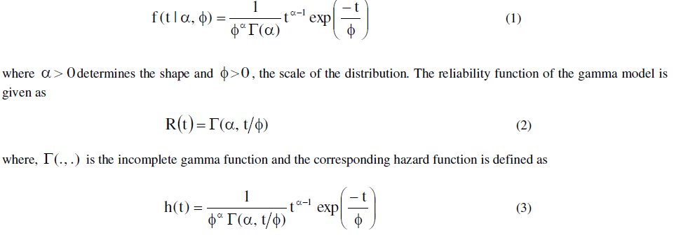
The parametric inference procedures for reliability data often involves distributions like weibull and exponential that have been widely accepted as important failure-time distributions. There are several other statistical models that can be successfully utilised for some particular types of data. The two-parameter gamma distribution is one of these probability distributions and is well suited for continuous, skewed responses. The gamma distribution fits a wide variety of failuretime data quite efficiently. Its relationship with the exponential distribution also has enhanced its importance as the sum of iid exponential random variables also follows gamma distribution. The pdf of gamma distribution is of the form

Although there is a vast literature available on estimation of the gamma parameters within the classical approach, we have worked here on the Bayesian inference of the gamma parameter(s). To evaluate characteristics of posterior such as densities, means and variances, is a very tedious task. When gamma model is used as a failure-time distribution, Bayesian computations become far more difficult as it involves incomplete gamma functions. Also, in the absence of conjugate priorlikelihood pair, evaluation of posterior quantities cannot be performed in closed forms and thus requires some intensive computational methods. As a solution to this, [1] proposed the use of Laplace's method to expectations and variances of non-positive functions.

The main aim of this paper is to demonstrate the fitting of gamma model in reliability scenario by employing Laplace's method in R [2]. The whole work is in data analytic context.

II. LAPLACE’S APPROXIMATION

The most remarkable method of evaluating integrals involved in the posterior density i.e

has been pioneered by Laplace and is known as Laplace method. [3] applied this method to approximate the ratio of two integrals involved in the posterior density. Contrary to [4], this method of summarizing multivariate posterior distribution needs only upto second-order derivatives of the posterior. The whole method is based on the behaviour of the posterior about it mode. Let ) ( h θ be any non-negative unimodal function with mode θˆ . We expand log h(θ) in a second-order Taylor series about θˆ as below,

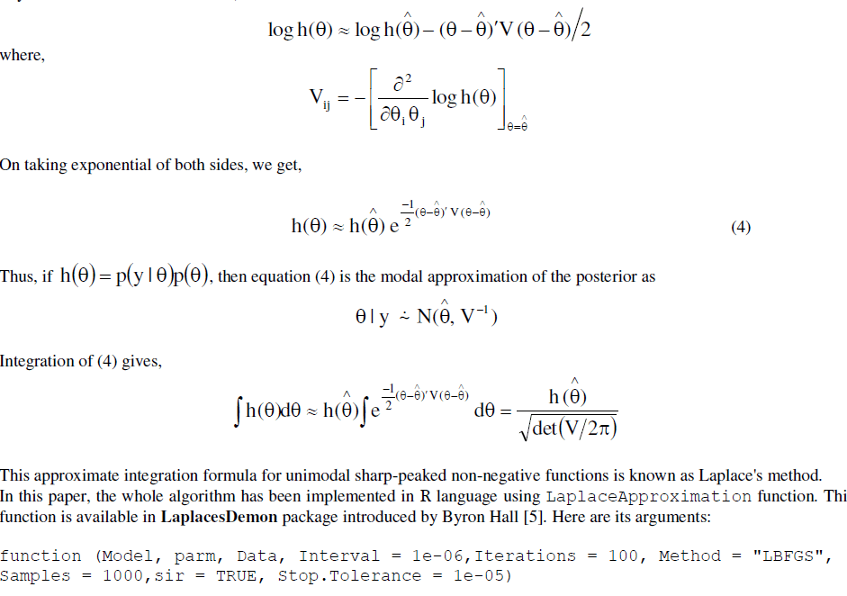where Model receives the model from a user-defined function. The argument parm requires a vector of initial values for the parameters for optimization. Data accepts a listed data object on which the model is to be fitted. sir takes a logical value to specify whether sampling importance resampling is to be implemented or not. It is implemented via SIR function of this package to draw independent posterior samples. The function LaplaceApproximation calls optim to maximize the logarithm of unnormalized joint posterior density. The default optimization algorithm is LBFGS. This function returns two summaries as Summary 1 and Summary 2. Summary 1 is the laplace approximation of the joint posterior density and Summary 2 presents the posterior means, sd and quantiles of all the parameters based on monte carlo samples.

III. SIMULATION

Another alternative to evaluate complex integrals is to resort to simulation technique. In the simplest cases, direct simulation and rejection sampling can be used. In complex situations, we apply Monte carlo and MCMC methods. Here, the function LaplacesDemon serves our purpose. The performance of the laplace approximation has been investigated through the simulation study. With the optimal initial values and estimated covariance matrix obtained from Laplace approximation, LaplacesDemon function maximizes the logarithm of unnormalised joint posterior density with MCMC. Arguments of this function are:

function (Model, Data, Initial.Values, Covar = NULL, Iterations =1e+05, Status = 1000, Thinning = 100, Algorithm = "RWM", Specs = NULL, ...)

where Model receives the same user-defined model, Data stands for the listed data object. Initial.Values accepts a vector of initial values supplied by LaplaceApproximation. Covar receives a dÃÂ¯ÃâÃÂ´d proposal covariance matrix (where d is the number of parameters) as returned by the function LaplaceApproximation. Iterations specifies the number of iterations that Laplace's Demon will update the parameters searching for target distribution. Algorithm reports the specific MCMC algorithm used for estimation and defaults to Random-Walk Metropolis algorithm.

IV. DATA ANALYSIS

In this section, we analyse a data from [6] to illustrate our methodology. The data involves failure times (in minutes) for a sample of 15 electronic components in an accelerated life test.

1.4, 5.1, 6.3, 10.8, 12.1, 18.5, 19.7, 22.2, 23.0, 30.6, 37.3, 46.3, 53.9, 59.8, 66.2

We now look for the posterior estimates of the parameters when the gamma model is fitted to the above data. The firstmost requirement for the Bayesian fitting is the definition of the likelihood. Here, we have likelihood as:

where,

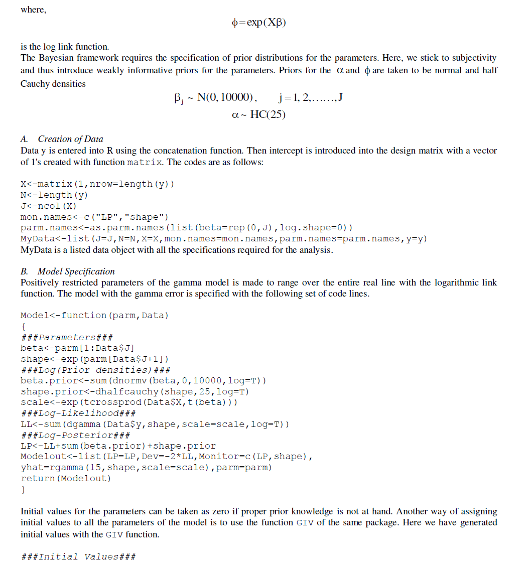Initial.Values<-GIV(Model,MyData,n=1000)

Finally, the fitting is done with the LaplaceApproximation function using the following commands ###Fitting with LaplaceApproximation### set.seed(1) M1<-LaplaceApproximation(Model,Initial.Values,MyData,Iterations=15000) Output summary has been tabulated in Table 1 and Table 2.

V. SIMULATION STUDY

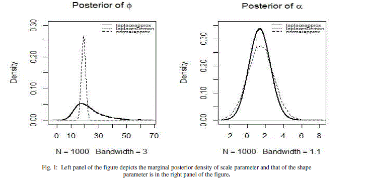
We implement Random-Walk Metropolis algorithm to simulate from the joint posterior distribution. A proposed future estimate called proposal of the joint target density is calculated and then the ratio of proposed to the current joint posterior density called α is calculated. The proposed state is accepted over the current state if the proposed state is an improvement over the current state. If the proposed state is rejected, then current state is repeated so that another proposal may be estimated at the next iteration. Here, the proposal distribution is multivariate normal. The whole process has been implemented using LaplacesDemon function. This function is however assisted by the function LaplaceApproximation. The R codes are as follows:

Initial.Values<-as.initial.values(M1) ###Fitting with LaplacesDemon### M11<-LaplacesDemon(Model,MyData,Initial.Values)

Output has been reported in Table 3.

VI. FAILURE TIME REGRESSION MODELING

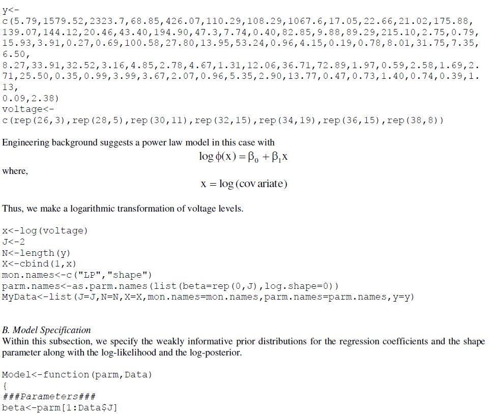
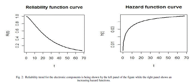
A model with explanatory variables (covariates) can sometimes best describe the heterogeneity in a population. It explains or predicts why some units survive a long time whereas others fail quickly. The main objective behind regression modeling is to exploit the relationship between failure-time and the explanatory variables. One of the way to create a regression model is to allow the model parameter(s) to depend on covariates. We illustrate this with insulating fluid failure-time data discussed by [7]. The data consists of breakdown times (in minutes) of 76 specimens of type of an electrical insulating fluid which were tested at seven voltage levels, v ÃÂ¯Ãâ¬ÃÂ½ 26, 28, 30, 32, 34, 36 kilovolts. The main objective of this study was to draw a relationship between time to breakdown and voltage stress.

A. Data creation

We create the data y in a vector form as below:

The same data has been studied through simulations. Here, the algorithm used is Adaptive-Mixture Metropolis. First, AMM updates a scatter matrix which is based on the cumulative current parameters and the cumulative associated outer-products, and these are used to generate a multivariate normal proposal. However, the proposal is a mixture. The two mixture components are adaptive multivariate and static/symmetric univariate proposals. At each iteration, the mixture is determined with a mixture weight. The mixture weight must be in the interval (0, 1], and it defaults to 0.05, as in [8]. A lower weight is associated with more adaptive multivariate proposals and a higher value of the mixture weight is associated with more static/symmetric univariate proposals. LaplacesDemon function has been used for this purpose. The R codes for it are as follows:

The parameter estimates are reported in Table 6.

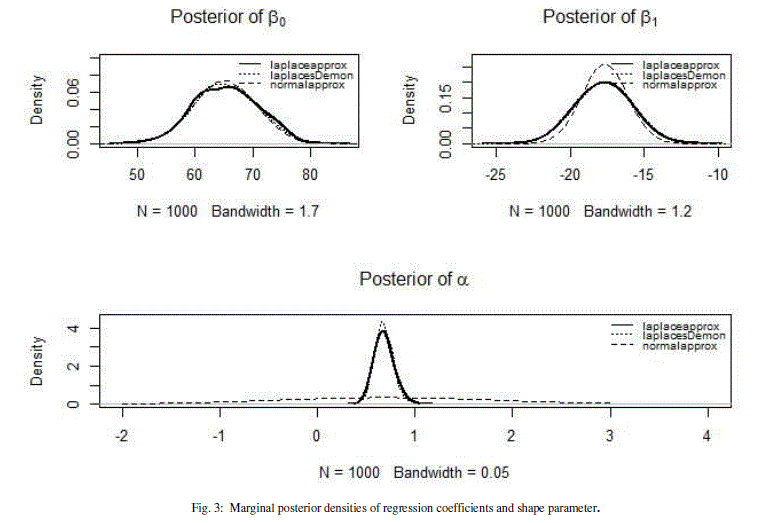
Based on the simulated values, marginal posterior densities of all the three parameters have been represented in Figure 3. The classical interpretation of density of parameter(s) estimates have been shown on the same plot.

VII. CONCLUDING REMARKS

This paper introduces the contributed R package LaplacesDemon that facilitates high dimensional Bayesian inference. It has been written entirely in R and has a remarkable provision for user-defined probability models. The main body of the article comprises of written and distributed codes for gamma modeling of real datasets with Laplace approximation. It has been found that Laplace approximation is a suitable alternative to the high-dimensional integrations and R provides a simple function namely LaplaceApproximation to implement it. Also, we have attempted to provide a true picture of the marginal posteriors in contrast to the one provided by the asymptotic theory of frequentist approach. It is evident from the results that Bayesian methods based on non-informative (or weakly-informative) priors are equally compatible to the classical methods of inference.

ACKNOWLEDGEMENT

The first author would like to thank University Grants Commission (UGC), New Delhi for financial assistance.

References

L. Tierney, R. E. Kass, J. B. Kadane, “Fully exponential Laplace approximations to expectations and variances of non-positive functions”, Journal of the American Statistical Association, Vol. 84, No. 407, pp. 710-716, 1989.
R Development Core Team, “R: A language and environment for statistical computing”, R Foundation for Statistical Computing, Vienna, Austria, 2012.
L. Tierney, J. B. Kadane, “Accurate approximations for posterior moments and marginal densities", Journal of the American Statistical Association, Vol. 81, No. 393, pp. 82-86, 1986.
D. V. Lindley, “Approximate Bayesian methods”, in Bayesian Statistics, eds. J. M. Bernardo. M. H. Degroot, D. V. Lindley, and A. M. F. Smith, Valencia, Spain: University Press, pp. 223-245, 1980.
Statisticat, LLC, LaplacesDemon: “Complete environment for Bayesian Inference”, R package version 13.03.04, URL http://www.bayesianinference. com, 2013.
J. F. Lawless, “Statistical Models and Methods for Lifetime Data”, Wiley, New York, 1982.
W. B. Nelson, “Statistical methods for accelerated lifetest data- the inverse power law model”, General Electric Co. Technical Report 71-C-011. Schenectady, New York, 1970a.
Roberts G, Rosenthal J, “Examples of Adaptive MCMC”, Computational Statistics and Data Analysis, 18, 349-367, 2009.
J. F. Lawless, “Statistical Models and Methods for Lifetime Data”, 2nd ed.,Wiley, New York, 2003.