Oluwadare O Ojo1*, Oluwaseun A Adesina2
1Department of Statistics, Federal University of Technology, Akure, Nigeria
2Department of Statistics, Ladoke Akintola University of Technology, Ogbomosho, Nigeria
Received: 22-May-2023, Manuscript No. JSMS-23-99594; Editor assigned: 24-May-2023, Pre QC No. JSMS-23-99594 (PQ); Reviewed: 07-Jun-2023, QC No. JSMS-23-99594; Revised: 25-Aug-2023, Manuscript No. JSMS-23-99594 (R); Published: 01-Sep-2023, DOI:10.4172/JSMS.9.4.001
Citation: Ojo OO, et al. Bayesian Estimation of Simultaneous Equation Models with Outliers and Multicollinearity Problem. RRJ Stats Math Sci. 2023;9:001.
Copyright: © 2023 Ojo OO, et al. This is an open-access article distributed under the terms of the Creative Commons Attribution License, which permits unrestricted use, distribution and reproduction in any medium, provided the original author and source are credited.
Visit for more related articles at Research & Reviews: Journal of Statistics and Mathematical Sciences
Outliers and multicollinearity are problems in the analysis of Simultaneous Equation Model (SEM). They can lead to bias or inefficiency of estimators. This study employed a Bayesian technique for estimation of SEM that is characterized with both multicollinearity and outliers. Monte Carlo experiment was applied while the data sets with specified outliers and multicollinearity were simulated for the SEM. The estimates of Bayesian and classical methods namely; two Stage Least Squares (2SLS), Three Stage Least Squares (3SLS), and Ordinary Least Squares (OLS) in simultaneous equation model were then compared. The criteria used for comparison were the Mean Square Error (MSE) and Absolute Bias (AB). The Bayesian method of estimation outperformed other classical methods followed by two stage least squares, three stage least squares, and limited information maximum likelihood in terms of MSE and AB. However, the classical method has the same performance with Bayesian method when there are no outliers and multicollinearity in the simultaneous equation model. Hence, Bayesian method of estimation is preferred than classical method when there is problem of outlier and multicollinearity in a just identified simultaneous equation model. Mathematical subject classification: 62C10, 62CO7.
Bayesian; Multicollinearity; Outliers; Monte Carlo; Simultaneous equation model
Researchers often face the problems of multicollinearity and outliers in applied works either planned or not planned. Multicollinearity and outliers can lead to poor predictive power of the model and statistical inferences. These can also lead to inefficiency of estimators of simultaneous equation model. When multicollinearity occurs in the simultaneous equation model, so many classical simultaneous equation estimators will be difficult to applied, especially the two stage least squares method. Outliers are typical observations that are greatly different from group of observations. They can also make the models to have high error rates and substantial distortions for both parameter and statistic estimates [1].
In recent times, attention has been given to the problem of outliers and multicollineaarity in both classical and Bayesian econometrics especially in regression models [2]. There is not so much research on outliers in simultaneous equation models but there are limited researches on multicollinearity in simultaneous equation models. Major works carried out on the outliers in simultaneous equation models are Mishra and Adepoju and Olaomi while researches on multicollinearity in simultaneous equation models are Schink and Chiu, Agunbiade and Iyaniwura, Agunbiade, Mishra, Ozbay and Toker [3].
Mishra proposed a robust method that generalizes the two Stage Least Squares (2SLS) to the Weighted two Stage Least Squares (W2SLS) to tackle the effect of outliers and perturbations in data matrix. Monte Carlo method experiment was conducted to examine the performance of the proposed method in simultaneous equations. It was found out that the robustness of the proposed method did not disrupt the magnitude of outliers but sensitive to the number of outliers in the data matrix [4].
The performance of five estimators; Ordinary Least Squares (OLS), two Stage Least Squares (2SLS), three Stage Least Squares (3SLS), Generalized Method of Moment (GMM), and Weighted two Stage Least Squares (W2SLS) of simultaneous equations model parameters with first order autocorrelation levels of error terms and there is outliers in the data at small sample sizes were considered by Adepoju and Olaomi. It was observed that the system method performed better than the single equation for all the cases of outliers considered [5].
Agunbiade and Iyaniwura investigated the performance of six different estimation techniques of a just identified simultaneous three equation model with three multi collinear exogenous variables. The estimators considered under the three levels of multicollinearity were Ordinary Least Squares (OLS), two Stage Least Squares (2SLS), three Stage Least Squares (3SLS), Limited Information Maximum Likelihood (LIML), Full Information Maximum Likelihood (FIML), and Indirect Least Squares (ILS). It was revealed that 2SLS, LIML and ILS estimators were the best for lower open interval negative level of multicollinearity while FIML and OLS were best for closed interval and upper categories level of multicollinearity [6].
Agunbiade investigated effect of multicollinearity and sensitivity of three estimators in three just identified simultaneous equation model with the aid of Monte Carlo approach. The study was estimates using mean of estimates and its bias. However, the study revealed that identical estimates as the assumed parameter was not produced but some estimates are quite close. The use of shapely value regression at the second stage of two-stage least squares for simultaneous equation when there is collinearity was also proposed by Mishra. It was observed that all the structural coefficients estimated with the proposed two-stage least squares have an expected sign and can help to overcome the problem of collinearity [7].
A biased estimation method was proposed by Ozbay and Toker to remedy the problem of multicollinearity that exists in simultaneous equations model. Two parameter estimation in linear regression model is carried out to the simultaneous equations model. Monte Carlo experiment and real life data were used to evaluate the proposed method. The performance of the estimation of the new method is better than the conventional two stage least squares estimator [8].
Many researchers have provided alternative solutions like M-estimator for outliers. However, these methods cannot be applied to outlier and multicollinearity when they occur in the data at the same time. In this study, we consider the two problems together, that is, multicollinearity and outliers in simultaneous equation model by using a Bayesian method of estimation. The performance of Bayesian method will be then be compared with some classical Simultaneous equation methods in the presence of outlier and multicollinearity [9,10].
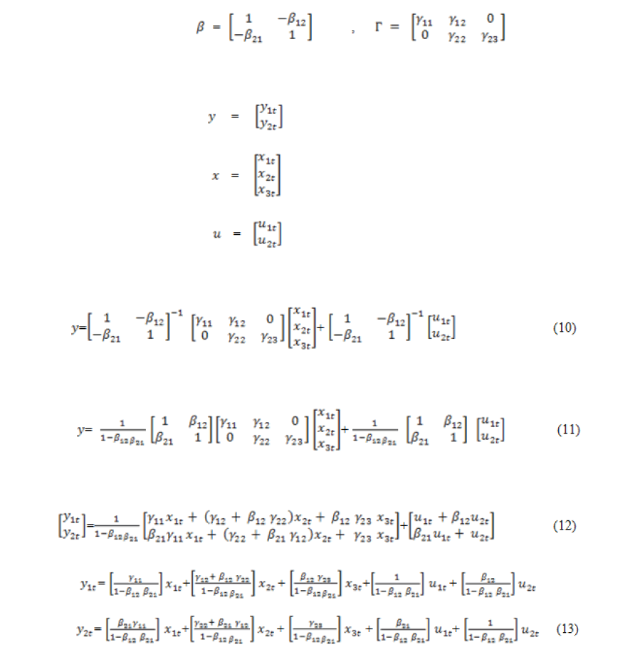
Consider the following two equations structural model;
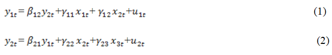
Where, y1t and y2t are the endogenous variables at time t and x1t,x2t and x3t are the exogenous or predetermined variables. The u1tand u2t are the random disturbance terms assumed to be independently and identically normally distributed with zero means and finite variance-covariance matrix Σ i.e., u~NID(0,Σ). Also β12, β21, γ11, γ12, γ22 and γ23 are unknown population parameters of the model.
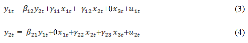
In this section, Bayesian method for solving multicollinearity and outlier problems will be given while different classical methods of solving simultaneous equation will be examined. The simultaneous equations given in (1) and (2) can further also be written as:
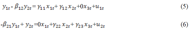
Rearranging, we have;
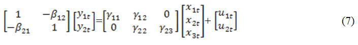
In matrix form;
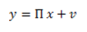
This can be written in reduced from as:
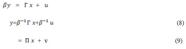
Where
Classical methods
Ordinary Least Squares (OLS): This method can be applied in regression model. If OLS is applied to an equation in a simultaneous model, there will usually be more than one current endogenous variable in a relation, and whichever variable is selected as dependent variable, the remaining endogenous variables which are correlated with the disturbance term will appear in the equation as explanatory variables. Hence, OLS estimates will be biased and inconsistent when used in simultaneous equation model, but will be applied in this study for comparison purpose [11].
Two Stage Least Squares (2SLS): This method is the most common method used for estimating simultaneous equation models. It was developed by Theil and independently by Basmann. It is applicable to equations, which are over identified or exactly identified and it is a single equation method, being applied to one equation of the system at a time. It is to eliminate the simultaneous equation bias [12].
Three Stage Least Squares (3SLS): It is a systems method, that is, it is applied to all the equations of the model at the same time and gives estimates of all the parameters simultaneously. This method was developed by Theil and Zellner as a logical extension of Theil’s 2SLS. It involves the application of the method of Least Squares in three successive stages. It utilizes more information than the single-equation techniques, that is, it takes into account the entire structure of the model with all the restrictions that the structure imposes on the values of the parameters [13].
Limited Information Maximum Likelihood (LIML): This is a single equation method which makes use of the principle of Maximum Likelihood. It is a “limited information” method because it does not make full use of the information provided by the equations of the model other than those of the particular equation under consideration. The limited information it requires on the other equations of the model, is the specification of all the truly exogenous variables that are contained in those other equations. It is an appropriate method for estimating over identified models [14].
Bayesian method
In Bayesian method, it is better to work on reduced form rather than the structural form due to prior elicitation and identification problem.
Recall from equation (9),
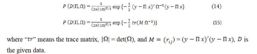
The likelihood function is the principal to the process of estimation of unknown parameters in Bayesian analysis. Using the definition of multivariate Normal distribution, the likelihood can be written as:
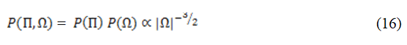
Prior distribution
When there is absence of prior knowledge, using a non-informative prior in Bayesian inference can be of great value. Here, we use a diffuse prior introduced by Jeffreys, which is given as:
Posterior distribution
The posterior distribution summarizes what we know about uncertain quantities. It gathers all the evidence or information that has been taken into account by prior distribution. Hence, it combines both the likelihood and prior distribution [15].
Therefore, the joint posterior density is proportional to the likelihood times prior and can simply be written as:
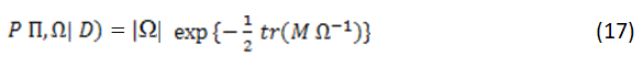
While the conditionals densities forms are given in equations (18) and (19):
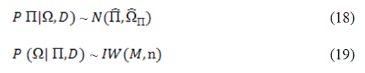
Equations in (18) and (19) are normal and inverse Wishart distributions
In order to obtain the point estimate from the posterior density functions, we will solve the conditional posteriors given in equations (18) and (19), these can be achieved by using the widely used method called Markov Chain Monte Carlo (MCMC).
Monte Carlo experiment
In this section, a Monte Carlo experiment will be setup to facilitate comparison between the Bayesian method and classical methods in simultaneous equation model that is characterized by multicollinearity and outliers. The steps of the experiment are outlined below:
• Generate the exogenous variables x1t,x2t and x3t for each sample point. Here, the variables will be generated from the uniform distribution (0,1) Kmenta and Ojo and Adepoju. These exogenous variables are characterized by multicollinearity and outliers. The levels of multicollinearity are:
High Multicollinearity (HM): 0.95 and 0.99
Low Multicollinearity (LM): 0.2, and 0.40
While the scenarios of outliers are: 0%, 10% and 20%
• The initial values of the parameters are chosen arbitrarily given as: β21=0.5, β;12=0.8, γ11=1.5, γ12=1.0, γ22
=1.0, γ23=1.0
• The disturbance terms, u1t and u2t will also be generated at each sample point.
• The disturbance terms and exogenous variables will be used to generate the endogenous variables.
• The sample sizes considered are 15, 50, and 100 while each of the samples is replicated 10000 times.
This Section discusses the results from the Monte Carlo experiment described in section 4. The MSE and ABIAS for estimators namely; Bayesian, two stage least squares, three stage least squares, limited information maximum likelihood, and ordinary least squares are obtained in Tables 1 and 2. It was observed that the estimates of two stage least squares, three stage least squares, and Limited information Maximum likelihood are the same, hence they are represented by 23LIML while Bayesian is represented by Bayes [16].
| Sample size | 15 | 50 | 100 | ||||||||
|---|---|---|---|---|---|---|---|---|---|---|---|
| Eqn | Method | Collinearity levels | Outliers | Outliers | Outliers | ||||||
| 0 | 10 | 20 | 0 | 10 | 20 | 0 | 10 | 20 | |||
| 1 | OLS | 0.99 | 2.056 | 2..353 | 2.436 | 1.665 | 1.814 | 1.921 | 1.451 | 1.513 | 1.613 |
| 0.6 | 0.714 | 0.913 | 1.274 | 0.501 | 0.61 | 0.736 | 0.247 | 0.426 | 0.51 | ||
| 0.2 | 0.561 | 0.61 | 0.402 | 0.492 | 0.592 | 0.72 | 0.158 | 0.013 | 0.218 | ||
| 23LIML | 0.99 | 1.583 | 1.393 | 1.691 | 1.329 | 1.489 | 1.391 | 0.481 | 0.821 | 0.942 | |
| 0.6 | 0.492 | 0.691 | 1.024 | 0.392 | 0.529 | 0.492 | 0.192 | 0.291 | 0.482 | ||
| 0.2 | 0.329 | 0.492 | 0.692 | 0.382 | 0.182 | 0.321 | 0.018 | 0.128 | 0.181 | ||
| Bayes | 0.99 | 0.197 | 0.192 | 1.283 | 0.732 | 0.821 | 0.913 | 0.002 | 0.148 | 0.285 | |
| 0.6 | 0.219 | 0.271 | 0.294 | 0.031 | 0.059 | 0.071 | 0.001 | 0.081 | 0.103 | ||
| 0.2 | 0.004 | 0.019 | 0.028 | 0.008 | 0.004 | 0.017 | 0.001 | 0.019 | 0.027 | ||
| 2 | OLS | 0.99 | 5.356 | 6.153 | 6.913 | 4.414 | 4.81 | 5.012 | 3.014 | 4.028 | 4.821 |
| 0.6 | 4.829 | 4.914 | 5.018 | 3.091 | 4.191 | 4.391 | 2.018 | 2.918 | 3.048 | ||
| 0.2 | 3.829 | 3.991 | 4.192 | 3.012 | 3.291 | 4.014 | 1.041 | 2.492 | 2.563 | ||
| 23LIML | 0.99 | 0.356 | 0.356 | 0.356 | 0.465 | 0.821 | 0.917 | 0.618 | 0.7183 | 1.632 | |
| 0.6 | 0.271 | 0.483 | 0.282 | 1.593 | 1.829 | 2.491 | 0.392 | 0.219 | 0.192 | ||
| 0.2 | 0.282 | 0.193 | 0.493 | 0.192 | 1.452 | 1.823 | 0.138 | 0.319 | 0.218 | ||
| Bayes | 0.99 | 0.008 | 0.013 | 0.21 | 0.013 | 0.029 | 0.193 | 0.001 | 0.021 | 0.043 | |
| 0.6 | 0.142 | 0.004 | 0.103 | 0.002 | 0.081 | 0.093 | 0.02 | 0.028 | 0.033 | ||
| 0.2 | 0.01 | 0.029 | 0.031 | 0.028 | 0.033 | 0.076 | 0.001 | 0.001 | 0.001 | ||
Table 1. Absolute Bias of the estimators with varying sample sizes for collinearity and outliers.
| Sample size | 15 | 50 | 100 | ||||||||
|---|---|---|---|---|---|---|---|---|---|---|---|
| Eqn | Method | Collinearity levels | Outliers | Outliers | Outliers | ||||||
| 0 | 10 | 20 | 0 | 10 | 20 | 0 | 10 | 20 | |||
| 1 | OLS | 0.99 | 6.192 | 7.396 | 7.921 | 4.019 | 5.829 | 6.183 | 2.029 | 2.712 | 2.098 |
| 0.6 | 4.193 | 5.94 | 6.011 | 3.983 | 3.391 | 3.017 | 1.393 | 2.001 | 3.191 | ||
| 0.2 | 5.193 | 5.812 | 5.889 | 2.001 | 2.397 | 4.191 | 1.43 | 1.552 | 2.083 | ||
| 23LIML | 0.99 | 4.289 | 4.908 | 4.716 | 1.933 | 4.882 | 5.018 | 0.255 | 1.38 | 0.829 | |
| 0.6 | 2.392 | 3.11 | 3.814 | 2.91 | 2.816 | 2.914 | 0.133 | 1.231 | 0.383 | ||
| 0.2 | 2.135 | 3.022 | 3.007 | 2.136 | 2.49 | 3.025 | 0.582 | 0.8 | 1.227 | ||
| Bayes | 0.99 | 1.669 | 1.382 | 1.888 | 1.216 | 1.305 | 1.529 | 0.501 | 0.628 | 0.723 | |
| 0.6 | 1.302 | 1.811 | 1.906 | 1.237 | 2.192 | 1.724 | 0.021 | 1.15 | 0.158 | ||
| 0.2 | 0.628 | 2.82 | 2.977 | 2.243 | 1.428 | 2.518 | 0.281 | 0.778 | 0.993 | ||
| 2 | OLS | 0.99 | 8.16 | 8.936 | 7.522 | 7.461 | 7.722 | 4.206 | 4.119 | 4.296 | 2.911 |
| 0.6 | 5.993 | 7.2 | 6.293 | 3.916 | 5.229 | 3.193 | 2.104 | 3.888 | 1.948 | ||
| 0.2 | 3.813 | 4.001 | 4.729 | 2.917 | 3.914 | 4.285 | 1.395 | 1.732 | 0.813 | ||
| 23LIML | 0.99 | 4.359 | 0.356 | 0.356 | 3.465 | 4.028 | 3.281 | 2.001 | 2.875 | 1.377 | |
| 0.6 | 3.006 | 4.913 | 0.182 | 1.11 | 2.913 | 2.015 | 1.393 | 1.118 | 0.724 | ||
| 0.2 | 1.842 | 3.927 | 1.996 | 2.537 | 2.114 | 2.439 | 0.832 | 1.027 | 1.279 | ||
| Bayes | 0.99 | 0.629 | 0.669 | 0.703 | 0.518 | 0.592 | 0.551 | 0.281 | 0.319 | 0.402 | |
| 0.6 | 0.382 | 0.49 | 0.511 | 0.317 | 0.423 | 0.518 | 0.201 | 0.289 | 0.318 | ||
| 0.2 | 0.029 | 0.201 | 0.388 | 0.026 | 0.173 | 0.192 | 0 | 0.001 | 0.016 | ||
Table 2. MSE of the estimators with varying sample sizes for collinearity and outliers.
From Table 1, the Bayes method has the least absolute bias followed by 23SLS while the OLS method has the largest absolute bias for the two equations for all the levels of collinearity. It was also observed that the bias estimates decreases the sample sizes increases for all the methods considered across the levels of collinearity. The ABIAS obtained in both equations 1 and 2 for 10% and 20% are higher than when there no outlier [17-20]. The ABIAS estimates for equation 1 are smaller than equation 2 for all the sample sizes considered across both levels of outliers and collinearity [21].
In Table 2, it is observed Bayes method gives the minimum MSE for the entire sample sizes considered followed by 23LIML while OLS has the highest MSE. All the methods are not greatly affected by outliers; however when the percentage of contamination goes to 10% and 20%, the MSE of the estimators increases. For low level of collinearity, the MSE are minimal.
Multicollinearity and outliers are great problems in applied work. This work determined the best method of estimation when a just identified simultaneous equation model has both problem of multicollinearity and outliers. The method considered were Bayesian, two stage least squares; three stage least squares, and Limited information maximum likelihood. When there is no outliers, all the estimators have the same performances, however when the levels of outlier were 10% and20%, the estimates of the estimators increases. The Absolute bias and Mean squared estimates of the estimators increases as the level of collinearity also increases. Also, all the methods considered show consistent asymptotic pattern with values of absolute bias and mean squared error decreasing consistently. Bayesian method of estimation is considered the best estimator when a just identified simultaneous equation model has both problem of multicollinearity and outliers.
There is no conflict of interest
There is no funding.
[Crossref] [Google Scholar] [PubMed]