Best Project Selection of Student?s through Rough Set, Bayes? Theorem Approach and Conflict Analysis

Abstract

This article based on project selection procedure of student with help of rough set approach insight into Bayes‟ theorem which help to compute to prior or posterior probabilities structure of the data being analyzed through which can draw conclusion of data and also compute the relationship in between Bayes‟ theorem and flow graph[11] and the granularity or conflict analysis of data can be represented in a form of a flow graph , and the relation between granules obeys Bayes‟ theorem that leads a new relation of data of decision table[12,13,16].

Keywords

Rough Set, Bayes‟ Theorem, Flow Graph, Conflict Analysis.

INTRODUCTION OF ROUGH SET

Rough set theory is a new mathematical approach to imperfect knowledge. The problem of imperfect knowledge has been tackled for a long time by philosophers, logicians and mathematicians. Recently it became also a crucial issue for computer scientists, particularly in the area of artificial intelligence. There are many approaches to the problem of how to understand and manipulate imperfect knowledge. The most successful one is, no doubt, the fuzzy set theory proposed by Zadeh [2].Rough set theory proposed by the author in [1] presents still another attempt to this problem. The theory has attracted attention of many researchers and practitioners all over the world, who contributed essentially to its development and applications

INDISCRENIBILITY MATRIX

Let I=(U, A) be an information system (attribute-value system), where „U‟ is a non-empty set of finite objects (the universe) and „A‟ is a non-empty, finite set of attributes such that a :U Va for every aA. „Va‟ is the set of values that attribute „a‟ may take. The information table assigns a value a(x) from „Va‟ to each attribute „a‟ and object „x‟ in the universe „U‟ with any B  Athere is an associated equivalence relationIND(B) [3,4,5,6].

Indiscrenibility-matrix is,

III. UPPER APPROXIMATION, LOWER APPROXIMATION & BOUNDARY REGION

The indiscrenibility relation will be used next to define approximations, basic concepts of rough set theory. Now approximations can be defined as follows: ,assigning to every subset X of the universe U two sets B*(X) and B*(X) called the B-lower and the B-upper approximation of X, respectively. The set will be referred to as the B-boundary region of X.

IV . INTRODUCTION OF BAYES’ THEOREM

The Bayes‟ theorem is the essence of statistical inference. The result of the Bayesian data analysis process is the posterior distribution that represents a revision of the prior distribution on the light of the evidence provided by the data” [7].“Opinion as to the values of Bayes‟ theorem as a basic for statistical inference has swung between acceptance and rejection since its publication on 1763” [8].Rough set theory offers new insight into Bayes‟ theorem [9]. The look on Bayes‟ theorem offered by rough set theory is completely different to that used in the Bayesian data analysis philosophy. It does not refer either to prior or posterior probabilities, inherently associated with Bayesian reasoning, but it reveals some probabilistic structure of the data being analyzed. It states that any data set (decision table) satisfies total probability theorem and Bayes‟ theorem. The Bayes‟ theorem is the essence of statistical inference.

V . INFORMATION SYSTEMS AND DECISION RULES

Every decision table describes decisions (actions, results etc.) determined, when some conditions are satisfied. In other words each row of the decision table specifies a decision rule which determines decisions in terms of conditions. In what follows we will describe decision rules more exactly.Let S = (U, C, D) be a

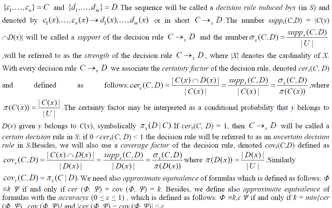An example of decision table shown in bellow Table1. In this table S1,S2,S3,S4,S5,S6 are students who are submitting their project and waiting for their selection, so, the selection procedure totally depended some conditions or criteria i.e. C1=Project field,C2=Project topic, C3=Project design, C4=Project implement, C5=Project performance. Table 1 illustrates the problem of finding the relationship between project selection conditions and decision conditions.

The example provided above that some decisions cannot be described by means of conditions.However, they can be described with some approximations. So,the approximation of above table 1 are [10]-

 The set {5} is lower approximation of the set {1,2,5} in which maximal set of facts that can be certainty classified as selection in term of conditions.

 The set {1,2,3,4,5} is upper approximation of the set {1,2,3,4,5,6} in which the set of facts that possibly can be classified as selection in term of conditions.

 The set {1,2,3,4} is boundary region of the set {1,2,3,4,5} in which the set of facts can be classified neither select nor reject of project in term of conditions.

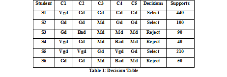
VII . COMPUTING STRENGTH , CERTAINTY COVERAGE FACTOR

for decision table are shown in Table 2.

Bellow a decision algorithm associated with Table 1 is presented.

1) If criteria C1 vgd & C4 gd then Decision→Select

2) If criteria C1 gd & C4 gd then Decision→Select

3) If criteria C1 gd & C4 md then Decision→Reject

4) If criteria C1 vgd & C4 bad then Decision→Reject

5) If criteria C4 vgd then Decision →Select

6) If criteria C4 bad then Decision→Reject

The certainty factor of the decision rules lead the following conclusion:

-94% student project have been selected .

-8% student project have been selected

-92% student project have been rejected.

-6% student project have been rejected.

-All student project have been selected.

-All student project have been rejected.

In other words :

-the most probability of select project 0.94 and 0.08 and all rejection probability 1.00 or selection probability 1.00.

Now let compute the inverse decision algorithm, which is given bellow :

1‟) If Decision→Select then criteria C1 vgd & C4 gd.

2‟) If Decision→Select then criteria C1 gd & C4 gd.

3‟) If Decision→Reject then criteria C1 gd & C4 md.

4‟) If Decision→Reject then criteria C1 vgd & C4 bad.

5‟) If Decision →Select then criteria C4 vgd.

6‟) If Decision→Reject then criteria C4 bad.

Now computing the inverse decision algorithm and the coverage factor we get the following explanation of decisions: -decision for select projects are most probability 0.10 if C1 vgd and C4 gd and decision for all select project probability is 0.11 if C4 is vgd.or probability for all reject project is 0.99.

VIII . FLOW GRAPH

So, with respect of rule 1 the condition C1 and C4 are approximately equivalent for selection project result where, k=0.89 and ε=0.81, and the C4 of project according to rule 3 is approximate equivalent to rejection result where, k=0.99, and ε=0.01 or selection result where, k=0.11, and ε=0.89.

IX . CONFLICT SPACE and CONFLICT GRAPH

With every decision table having one n-valued decision attribute we can associated n-dimensional Euclidean space where values of the decision attribute determine n axis of the space and condition attribute values (equivalence classes) determine point of the space. Strengths of decision rules are to be understood as coordinates of corresponding points[14,15].Distance  (x, y) between granules x and y in an n-dimensional decision space is defined as

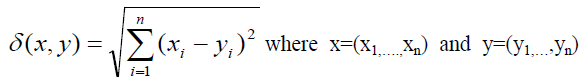are vectors of strength of corresponding decision rules[16].Conflict Space for Table 1 is shown in Fig 2:

So, the conflict graph or distances between granules (1,4),(2,3),(5),(6) are shown in bellow.

X . CONCLUSION

In this article, Bayes‟ theorem consists of prior or posterior probabilities and rough set approach to Bayes‟ theorem reveals data pattern, which normally used to draw conclusions from data in the form of decision rules[11]. Besides the rough set rules Bayes‟ approach invert rules for getting actual decision which shown in example in this article as well as it also help to associated to draw flow graph which gives a new tool to decision analysis.Besides, the relation between condition and decision granules are represented as flow graph and a conflict space is defined to analyze similarity of data granules[16].

References

1. Z. Pawlak: Rough sets, International Journal of Computer and Information Sciences, 11, 341-356, 1982
2. L. Zadeh: Fuzzy sets, Information and Control, 8, 338-353, 1965
3. Z. Pawlak (1991), Rough Sets “Theoretical Aspects of Reasoning about Data”.Kluwer Academic Publishers, Dordrecht.
4. Z. Pawlak: Rough sets, Int. J. of Information and Computer Sciences, 11, 5, 341-356, 1982
5. Z. Pawlak, A. Skowron: Rough membership function, in: R. E Yeager, M. Fedrizzi and J. Kacprzyk (eds.), Advaces in the Dempster-Schafer of Evidence, Wiley, New York, 1994, 251-271
6. L. Polkowski, A. Skowron: Rough mereological calculi granules: a rough set approach to computation, computational intelligence: An International Journal 17, 2001, 472-479
7. G. E. P. Box, G. C. Tiao: Bayesian Inference in: Statistical Analysis, John Wiley and Sons, Inc., New York, Chichester, Brisbane, Toronto, Singapore, 1992
8. M. Berthold, D. J. Hand: Intelligent Data Analysis, an Introduction, Springer-Verlag, Berlin, eidelberg, New York, 1999
9. Z. Pawlak: Rough Sets and Decision Algorithms, in: W. Ziarko, Y. Y. Yao (eds.), Second International Conference, Rough Sets and Current Trends in Computing, RSCTC 2000, Banff, Canada, October 2000, LNAI 2000, 30-45
10. Z. Pawlak:A Primer on Rough Set: A New Approach to Drawing Conclusions from Data.
11. Z. Pawlak: Bayes‟ Theorem – The Rough Set Perspective. Institute of Theoretical and Applied Informatics, Polish Academy of Sciences,ul. Ba_ltycka 5, 44 100 Gliwice, Poland.
12. Pawlak, Z. (1998). An Inquiry into Anatomy of Conflicts, Journal of Information Sciences, 109, 65-68.
13. Pawlak, Z. (2002). Rough Sets, Bayes' Theorem and Flow Graphs, IMPU 2002, To appear.
14. Slowinski, R. (1995). Rough Set Approach to Decision Analysis, AI Expert 10, 18-25.
15. “CONFLICTS AND DECISIONS”, Zdzis law Pawlak, University of Information Tehnology and Management ul. Newelska 6, 01 447 Warsaw, Poland.
16. Z.Pawlak, “Theorize with Data using Rough Sets”, University of Information Technology and Management, Newelska 6, 01 447 Warwaw, Poland