Keywords
|
| Genetic Programming, Support Vector Machine, Benign, Malignant |
INTRODUCTION
|
| Breast cancer is ranked first among the leading causes of cancer affecting female. Statistics have shown that one among ten women is affected by breast cancer in their life time. Detection and diagnosis of the disease at an earlier stage can ensure a long survival of lives. The symptoms of breast cancer include mass, changes in shape and dimension of breast. Various diagnostic tests and procedures are available for detecting the presence of breast cancer. One of these is analysis of a biopsy taken from the breast to identify the breast cancer. Several methods for a breast biopsy exist like Fine needle aspiration, Core needle biopsy, Vacuum assisted biopsy, Open surgical biopsy, etc to identify the breast cancer. The Fine Needle Aspiration (FNA) is a percutaneous procedure that uses a fine needle and a syringe to sample fluid from a breast cyst or remove clusters of cells from a solid mass. The samples of breast tissue are analysed using microscope and the result may be benign (non-cancerous cells) or Malignant (Cancerous cells). |
RELATED WORK
|
| Numerous methods and algorithms have been adopted on classification of breast cancer. Sarvestan Soltani, et al. provided a comparison among the capabilities of various neural networks such as Multilayer Perceptron (MLP), Self Organizing Map (SOM), Radial Basis Function (RBF) and Probabilistic Neural Network (PNN) which are used to classify WBC and NHBCD data. The performance of these neural network structures was investigated for breast cancer diagnosis problem. RBF and PNN classifier were proved as the best classifiers in the training set. This work showed that statistical neural networks can be effectively used for breast cancer diagnosis [1]. |
| Fogarty, et al. pre-processed data from the Wisconsin Diagnostic Breast Cancer (WDBC) is directly fed as terminal values to a genetic programming algorithm and the output of the algorithm is compared with the required output and the fitness computed. A population of individuals is generated and the best individuals are selected. The population converges to the solution that best represents the discrimination function and obtains a detection accuracy of 96.32% and compared their results of GP with many techniques namely MLP, General Regression, Radial Basis Function, Mixture of Experts, LDA, Logistic Regression, K Search Neighbour and Kernel for diagnosis of breast cancer [2]. |
| Iranpour, et al. discussed the application of Support Vector Machines (SVM), Radial Basis Function (RBF) networks for breast cancer detection and obtained an accuracy of 98.1% which is compared favourably to accuracies obtained in other studies like linear SVM classifier (94%), fuzzy classifiers (95.8%), and edited nearest neighbour with pure filtering (95.6%) [3]. |
| In the proposed work, breast cancer classification task carried out using Wisconsin Diagnostic Breast Cancer (WDBC) database which is a processed form of the Fine Needle Aspiration data. Genetic Programming and Support Vector Machine classifiers are used to perform classification. |
SUPPORT VECTOR MACHINE
|
| Support Vector Machine a new approach to supervised pattern classification which has been successfully applied to a wide range of pattern recognition problems. Support Vector Machine is a training algorithm for learning classification and regression rules from data. SVM is most suitable for working accurately and efficiently with high dimensionality feature spaces. SVM is based on strong mathematical foundations and results in simple yet very powerful algorithms [4-6]. |
| The standard SVM algorithm builds a binary classifier. A simple way to build a binary classifier is to construct a hyperplane separating class members from non-members in the input space. SVM also finds a nonlinear decision function in the input space by mapping the data into a higher dimensional feature space and separating it there by means of a maximum margin hyperplane. The system automatically identifies a subset of informative points called support vectors and uses them to represent the separating hyperplane which is sparsely a linear combination of these points. Finally SVM solves a simple convex optimization problem. |
| The machine is presented with a set of training examples, (xi, yi) where the xi are the real world data instances and the yi are the labels indicating which class the instance belongs to. For the two class pattern recognition problem, yi = +1 or yi = -1. A training example (xi, yi) is called positive if yi = +1 and negative otherwise. SVM construct a hyperplane that separates two classes and tries to achieve maximum separation between the classes. Separating the classes with a large margin minimizes a bound on the expected generalization error. |
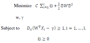
| The simplest model of SVM called Maximal Margin classifier, constructs a linear separator (an optimal hyperplane) given by w T x - γ = 0 between two classes of examples. The free parameters are a vector of weights w which is orthogonal to the hyperplane and a threshold value γ. These parameters are obtained by solving the following optimization problem using Lagrangian duality |
 |
| where Dii corresponds to class labels, which assumes value +1 and –1. The instances with non null weights are called support vectors. |
| In the presence of outliers and wrongly classified training examples it may be useful to allow some training errors in order to avoid overfitting. A vector of slack variables ξi that measure the amount of violation of the constraints is introduced and the optimization problem referred to as soft margin is given below |
 |
| The minimization of the objective function causes maximum separation between two classes with minimum number of points crossing their respective bounding planes. The parameter C is a regularization parameter that controls the trade-off between the two terms in the objective function. The proper choice of C is crucial for good generalization power of the classifier. The following decision rule is used to correctly predict the class of new instance with a minimum error. |
| The advantage of the dual formulation is that it permits an efficient learning of non–linear SVM separators, by introducing kernel functions. Technically, a kernel function calculates a dot product between two vectors that have been (nonlinearly) mapped into a high dimensional feature space. Since there is no need to perform this mapping explicitly, the training is still |
 |
| feasible although the dimension of the real feature space can be very high or even infinite. The parameters are obtained by solving the following non linear SVM dual formulation (in Matrix form), |
 |
| where Q=DKD and K is kernel matrix. The kernel function K(AAT) may be polynomial or RBF (Radial Basis Function) is used to construct hyperplane in the feature space, which separates two classes linearly, by performing computations in the input space. The decision function in this nonlinear case is given by |
 |
| where u, the Lagrangian multipliers. |
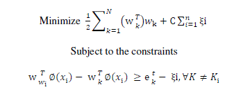
| When the number of classes is more than two, then the problem is called multiclass SVM. There are two types of approaches for multiclass SVM. In the first method called indirect method, several binary SVM’s are constructed and the classifier’s output are combined for finding the final class. In the second method called direct method, a single optimization formulation is considered. The formulation of one of the direct methods called Crammer and Singer Method is |
 |
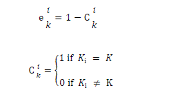
| where ki is the class to which the training data xi belong, |
 |
| The decision function for a new input data xi is given by |
 |
| where |
 |
GENETIC PROGRAMMING
|
| Genetic Programming (GP) is an evolutionary computation technique that automatically solves problems without requiring the user to know or specify the form or structure of the solution in advance. Genetic Programming evolves a population of computer programs. Generation by generation, GP stochastically transforms populations of programs into new, hopefully better, populations of programs. GP has been very successful at evolving novel and unexpected ways of solving problems. Genetic programs may be regarded as prediction models that approximate an objective function f: In → Om with In denotes the input data space of dimension n and Om is the m-dimensional output data space. In most cases there is only m = 1 output. Genetic programs may also complete missing (unknown) parts of an existing model. Other evolutionary algorithms, like genetic algorithms or evolution strategies, minimize an existing objective function (model) by searching for the optimum setting of its variables (model parameters). |
| The objective function itself represents the problem to be solved by GP. In practice this function is usually unknown, incompletely defined by a relatively small set of input-output vectors. The evolutionary process searches for a program that represents the best solution to a given problem. The genetic programs are desired to generalize from the training data to unknown data. |
| A. Linear Genetic Programming |
| LGP is a particular subset of genetic programming wherein computer programs in population are represented as a sequence of instructions from imperative programming language or machine language. The semantics of linear GP are quite different; instructions in LGP typically read their input from one or more registers or memory locations and store the results of their calculations in a register. Instructions in linear GP all have equivalent roles and communicate only via registers or memory. In linear GP there is no equivalent of the distinction between functions and terminals inherent in tree-based GP. The instructions in linear GP may be machine code GP, where each instruction is directly executable by the CPU, or interpreted linear GP, where each instruction is executable by some higher-level virtual machine typically written in an efficient language such as C / C++/ Java). The interpreted linear programs are slower than machine-code programs, but an interpreted linear GP system can be more efficient than an interpreted tree-based systems. |
| The basic steps in a Linear Genetic Programming are [7] |
| Step1: Randomly create an initial population of programs from the available primitives |
| Step 2: repeat |
| Step 3: Execute each program and ascertain its fitness |
| Step 4: Select one or two programs from the population with a probability based on fitness to participate in genetic operations |
| Step 5: Create new individual program by applying genetic operations with specified probabilities |
| Step 6: Until an acceptable solution is found or some other stopping condition is met (e.g., a maximum number of generations are reached). |
| Step 7: Return the best-so-far individual. |
| The Linear Genetic Programming involves the various operations like initializing the population, selection of programs based on fitness, applying genetic operations, parameter setting. The various tasks are elaborated below. |
| Initialization of population: Like other evolutionary algorithms, the individuals in the initial population are typically randomly generated in LGP. There are a number of different approaches in generating this random initial population like full and grow methods, Ramped half and half methods. |
| Selection of Individuals: As with most evolutionary algorithms, genetic operators in LGP are applied to individuals that are probabilistically selected based on fitness. That is, better individuals are more likely to have more child programs than inferior individuals. The most commonly employed method for selecting individuals in GP is tournament selection, but any standard evolutionary algorithm selection mechanism like fitness-proportionate selection, stochastic universal sampling can be used. |
| Linear GP Operators: GP departs significantly from other evolutionary algorithms in the implementation of the operators of crossover and mutation. Crossover operation creates a child program by combining randomly chosen parts from two selected parent programs. Mutation operation creates a new child program by randomly altering a randomly chosen part of a selected parent program. The typical crossover and mutation operators for linear GP ignore the details of the machine code of the computer being used. For example, crossover may choose randomly two crossover points in each parent and swaps the code between them. Since the crossed over fragments are typically of different lengths, such a crossover may change the programs' lengths. Since computer machine code is organized into 32- or 64-bit words, the crossover points occur only at the boundaries between words. Therefore, a whole number of words, containing a whole number of instructions are typically swapped over. Similarly, mutation operations normally respect word boundaries and generate legal machine code [8]. |
| Fitness Function: Usually fitness is derived from a mapping error between the predicted model and the desired model. Since, in general, fitness cases represent a fraction of the problem data space only; fitness may reflect the phenotype behaviour of a program only in part. Fitness evaluation of individuals is by far the most time-critical step of a GP algorithm since a genetic program has to be executed at least once for each fitness case in the fitness function. There is something unusual about the fitness functions used in GP that differentiates them from those used in most other evolutionary algorithms. Because the structures being evolved in GP are computer programs, fitness evaluation normally requires executing all the programs in the population, typically multiple times. While one can compile the GP programs that make up the population, the overhead of building a compiler is usually substantial, so it is much more common to use an interpreter to evaluate the evolved program. |
EXPERIMENT AND RESULT
|
| Breast Cancer classification work has been carried out using Wisconsin Diagnosis Breast Cancer dataset created by Dr. William H. Wolberg at the University of Wisconsin. This dataset consists of 569 observations of patients with breast cancer among which 357 are benign and 212 are malignant status. Each instance has 32 features including id number and the class label that correspond to the type of breast cancer benign or malignant. These features are computed from digital image of fine needle of aspirates (FNA) of breast masses that describes the characteristics of the cell nuclei in the image. |
| The proposed work performed as two experiments. The first experiment is carried out using SVM Light, open source tool for multi class SVM, which uses Crammer and Singer Method. Second experiment aimed at assessing the effectiveness of Genetic Programming using the tool Discipulus, commercial Genetic Programming and data analysis software which handles regression, classification, ranking and logistics problem. Discipulus generates computer programs automatically in C, Java, C Sharp, Delphi and Intel assembler code on a desktop computer. Discipulus handles binary classification tasks. Discipulus is bundled with Notitia, which performs operations that include importing data from external sources, cleaning-up, and transforming and splitting data for use in Discipulus. In both the experiments the training set consists of 80% of instances and testing set consists of 20% of instances of both benign and malignant classes. |
| The dataset is trained with Linear, Polynomial and RBF kernel of SVM with different parameter settings for Cregularization parameter. In case of polynomial and RBF kernels, the default settings for d (Degree of polynomial) and g (Degree of gamma) are used. The performance of the trained models is evaluated using 10-fold cross validation for its predictive accuracy. The performance of the SVM classifier is summarized in Table I. |
| The control parameters settings used in Discipulus for the LGP generation process are shown in Table II. |
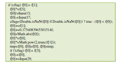
| The classifier generated after the specified number of runs are shown in Fig.1. |
| The program is converted into Java program and tested with test data set and the voting and confidence for each class is observed. The hit rate for benign and malignant class is presented in Table III. |
| From the results, it is observed that increasing number of runs in Discipulus tool provide substantial accuracy. Comparing with the performance of Support Vector Machine classifier, Evolutionary algorithm Linear Genetic Programming is significantly better in both prediction and training time. |
CONCLUSION
|
| This work demonstrates the modelling of breast cancer as classification task and describes the implementation of Support Vector Machine and Genetic programming approach for classifying breast cancer. Discipulus have been applied for generating LGP based classification models. It is observed that classification implemented by Genetic Programming in this paper is more efficient than other machine learning algorithms because the commercial GP software Discipulus uses automatic induction of binary machine code to achieve better performance. Effective models Copyright to IJIRCCE generated using linear genetic programming can be used by medical experts to classify the fine needle aspiration samples of breast tissue as benign or malignant and provide timely treatment. |
Tables at a glance
|
|
|
| |
Figures at a glance
|
 |
| Figure 1 |
|
References
|
- SarvestanSoltani A, Safavi A A, Parandeh M N and Salehi M , “Predicting Breast Cancer Survivability using Data Mining Techniques”,Software Technology and Engineering (ICSTE), 2nd International Conference, Vol.2, pages 227-231,2010.
- Werner J C and Fogarty T C, “Genetic Programming Applied to Severe Diseases Diagnosis”, In Proceedings Intelligent Data Analysis inMedicine and Pharmacology (IDAMAP), 2001.
- Iranpour M, Almassi S and Analoui M, “Breast Cancer Detection from fna using SVM and RBF Classifier”, In 1st Joint Congress on
- Fuzzy and Intelligent Systems, 2007.
- Joachims T, Scholkopf B, Burges C and Smola A, “Making large-scale SVM Learning Practical, Advances in Kernel Methods-SupportVector Learning”, Cambridge, MA, USA, 1999.
- Soman K P, Loganathan R and Ajay V, “Machine Learning with SVM and Other Kernel Methods”, PHI, India, 2009.
- CrammmerKoby and Yoram Singer, “On the Algorithmic Implementation of Multi-class Kernel-based Vector Machines”, Journal of
- Machine Learning Research, MIT Press, Cambridge, MA, USA, Vol.2, pages 265-292, 2001.
- Riccardo Poli, William B and Langdon Nicholas F McPhee, “A Field Guide to Genetic Programming”, Lulu Enterprises, UK, 2008.
- Markus Brameier and Wolfgang Banzhaf, “A Comparison of Linear Genetic Programming and Neural Networks in Medical Data
- Mining”, IEEE Transactions on Evolutionary Computation, Vol.5, Issue No.1, 2001.
|