International Journal of Advanced Research in Electrical, Electronics and Instrumentation Engineering
ISSN ONLINE(2278-8875) PRINT (2320-3765)
ISSN ONLINE(2278-8875) PRINT (2320-3765)
P.Venkatesh1, Dr .V.C.Veera Reddy2, Dr T.Ramashri3
|
| Related article at Pubmed, Scholar Google |
Visit for more related articles at International Journal of Advanced Research in Electrical, Electronics and Instrumentation Engineering
Basically beam splitters are used to capture RGB image in digital cameras, which is very expensive. This paper proposes an inexpensive technique using color filter arrays instead of beam splitters in digital cameras. Color filter arrays are inexpensive because it uses single sensor to capture multi color information unlike beam splitters (which contains multi sensors). Single sensor digital cameras captures only one at each pixel location and the other two color information to be interpolated is called Color Filter Array (CFA) interpolation or demosaicking. Demosaicking of process is estimated using color difference/ ratio rule of an RGB image. After demosaicking to reduce the noise in the interpolated images, adaptive filter is used. Adaptive filter is preferred since it provides better performance in texture and edge regions of interpolated images by removing interpolation errors. The performance of developed algorithm “CFAI using adaptive filter” is evaluated using PSNR, which is calculated between captured image and interpolated image. Thus it is observed that the proposed algorithm is more robust with high PSNR.
| RGB image ,Color filter array interpolation (CFAI), Color demosaicking, Adaptive filter, Color difference/ ratio rule and PSNR. |
||||||||||||||||||
INTRODUCTION |
||||||||||||||||||
| The common approach in single-chip digital cameras is to use a color filter arrays (CFA) to sample different spectral components like red, green, and blue. In the CFA - based sensor configuration, only one color is measured at each pixel location and the missing two color values are estimated. The estimation process is known as color demosaicking. The resulting image is a gray-scale mosaic-like one. Demosaicking algorithm interpolates sets of complete red, green, and blue values for each pixel, to make an RGB image [1]. Independent interpolation of color channels usually leads to drastic color distortions. The way to effectively produce a joint color interpolation plays a crucial role for demosaicking [2]. Modern efficient algorithms exploit several main facts. The first is the high correlation between the red, green, and blue channels for natural images. As a result, all three color channels are very likely to have the same texture and edge locations. The second fact is that digital cameras use the CFA in which the luminance (green) channel is sampled at the higher rate than the chrominance (red and blue) channels [3]. Therefore, the green channel is less likely to be aliased, and details are preserved better in the green channel than in the red and blue channels. Also, the CFA is a crucial element in design of single-sensor digital cameras. Different characteristics in design of CFA affect both performance and computational efficiency of the demosaicking solution .The fundamentals about digital color image acquisition with single-sensor can be found in. Cost effective digital cameras use a single-image sensor, applying alternating patterns of red, green, and blue color filters to each pixel location. The problem of reconstructing a full three-color pixel representation of color images by estimating the missing pixel components in each color plane is called demosaicking. Most existing demosaicking algorithms are heuristic algorithms. Bilinear interpolation (BI) is the simplest heuristic method, in which the missing samples are interpolated on each color plane independently and high frequency information cannot be preserved well in the output image [5]. With the use of inter-channel correlation, algorithms proposed in [8],[11]. Attempt to maintain edge detail or limite hue transitions to provide better demosaicking performance. In [12], an effective color interpolation method is proposed to get a full color image by interpolating the color differences between green and red/blue plane. A color-ratio model or a color-difference model cooperating with an edge-sensing mechanism is used to derive the interpolation process along the edges [14]. While, in [16], an adaptive demosaicking scheme using bilateral filtering technique is proposed. The demosaicking algorithm interpolate sets of complete red, green and blue values for each pixel, to make an RGB image. It is better than previous methods. |
||||||||||||||||||
| 1.1 Correlation Models | ||||||||||||||||||
| There are two basic inter plane correlation models. | ||||||||||||||||||
| 1.1.1 Color Difference Rule: | ||||||||||||||||||
| The first model asserts that intensity differences between red, green, and blue channels are slowly varying, that is the differences between color channels are locally nearly constant. Thus, they contain low-frequency components only, making the interpolation using the color differences easier. |
||||||||||||||||||
| 1.1.2 Color Ratio Rule: | ||||||||||||||||||
| The second correlation model is based on the assumption that the ratios between colors are constant over some local regions. This hypothesis follows from the Lambert’s law that if two colors have equal chrominance then the ratios between the intensities of three color components are equal . |
||||||||||||||||||
| The remaining paper is organized as follows: In section ‘2’ presents the brief overview of CFAI. In section ‘3’describes the proposed interpolation method. In section ‘4’ explains the experimental results and Section ‘5’ in reports the conclusions. |
||||||||||||||||||
OVERVIEW OF CFA INTERPOLATION |
||||||||||||||||||
| In the proposed work, digital cameras captures only one color information of the required three color samples becomes available at each pixel location and the other two color information to be interpolated is called Color Filter Array (CFA) interpolation or demosaicking. |
||||||||||||||||||
| There are various non adaptive CFA interpolation algorithms, these are nearest neighbor interpolation, bilinear interpolation, Smooth Hue Transition. The simplest algorithm for demosaicking is nearest neighbor. Nearest neighbor assigns a color value with the nearest known red, green or blue pixel value in the same color plane. There is usually some ordering as to which nearest neighbor to use (left, right, top, or below) for the particular implementation. However, it does not do a good job of interpolation, and it creates zig-zag zipper color artifact that distort the image. |
||||||||||||||||||
| Bilinear interpolation goes one step further from Nearest Neighbor Interpolation by taking the average value of all the nearest neighbors. For interpolation of red/blue pixels at a green position, the average of the two adjacent pixels of the same color is assigned to the interpolated pixel. |
||||||||||||||||||
PROPOSED WORK |
||||||||||||||||||
| The proposed algorithm is an improvement over I.Pekkucuksen et al method[1]. And the adaptive filter concept has been adopted from[3]. The developed algorithm consists of mainly three concepts; they are initialization, filtering and interpolation. Initialization is used to approximate and estimate color components, from which directional differences between G-R and G-B color channels are calculated. The noise present in these channels is filtered using adaptive filter. Finally, interpolation of pixels of an image is obtained by calculating missing color values at each pixel location. |
||||||||||||||||||
| 3.1 Initialization | ||||||||||||||||||
| Firstly, calculated the directional (horizontal and vertical) estimates of the green channel at every point ((i,j) X) in entire image. The interpolation of G color channel at R positions ((i,j) XR) is done as follows: |
||||||||||||||||||
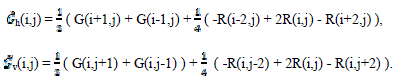 (1) (1) |
||||||||||||||||||
| (1)Here, h and v stand for horizontal and vertical estimates. find out the initial directional estimates for the red channel R and blue channel B at the green positions G (i,j) similar way to proceed shown above the equation (1). |
||||||||||||||||||
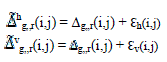
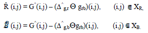
| At every point, the differences between the true values R(i,j) and G(i,j) and the directional estimates h(i,j) and h(i,j) are calculated as follows: |
||||||||||||||||||
 (2) (2) |
||||||||||||||||||
| g,r(i,j) are the directional differences between green and red color channels. | ||||||||||||||||||
 (4) (4) |
||||||||||||||||||
| Where Ãâ ÃÂh(i,j) and Ãâ ÃÂv(i,j) are considered as random demosaicking noises in horizontal and vertical directions. Δg,r(i,j) is the true difference between green and red color channels. The blue channel B is treated in the same way, and calculated the directional differences |
||||||||||||||||||
| 3.2 Filtering of Directional Differences | ||||||||||||||||||
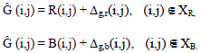
| The LPA-ICI filtering is used for all noisy estimates Δh g,r(i,j), Δv g,r(i,j) for R, and Δh g,b(i,j), Δv g,b(i,j) for B. Introduce this filtering in the form applicable for any input data, here assumed for a moment that this input noisy data have the form: |
||||||||||||||||||
| where (i,j) X, z(i,j) is a noisy observation, y(i,j) is a true signal and n(i,j) is a noise information. The LPA is a general tool for linear filter design, in particular for design of the directional filters of the given orders on the arguments i and j. Let gs,y be the impulse response of the directional linear filter designed by the LPA. Where y is a direction of smoothing and s is a scale parameter (window size of the filter). The details of the filter design are the exploited linear filter is obtained as a linear combination of two1D filters: |
||||||||||||||||||
| Where g0 s,Ãâé is a zero-order polynomial kernel, g1 s,Ãâé is a first-order polynomial kernel, and s is the length of the filters. The mixing parameter α is fixed to be 0.1 in this article. Approximation with larger than zero-order often results in higher instability of filtering, while zero-order often results in lower performance. Therefore, exploited a combination of zero- and first-order kernels. A set of the image estimates of different scales s and different directions θ are calculated by the convolution. |
||||||||||||||||||
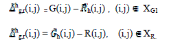
| 3.3.1 Interpolation of G Color | ||||||||||||||||||
| The interpolation green color channel at R((i,j) XR) and B((i,j) XB) positions are calculated as follows: | ||||||||||||||||||
 (8) (8) |
||||||||||||||||||
| Where Δg,r and Δg,b are the directional estimates of G–R and G–B color channels. | ||||||||||||||||||
| 3.3.2 Interpolation of R/B Colors at B/R Positions | ||||||||||||||||||
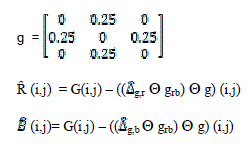
| For the interpolation of R/B colors at B/R positions, here proposed a method to use a special shift-invariant interpolation filter giving the estimates by the standard convolution. This filter has been designed using the LPA for the sub sampled grid, which corresponds to R/B channel (Fig. 1) with the symmetrical window function. A variety of polynomial orders and support sizes has been tested. Finally, the second-order polynomial interpolation filter grb has been chosen. |
||||||||||||||||||
| Then, the interpolated estimates are computed as follows: | ||||||||||||||||||
 (9) (9) |
||||||||||||||||||
| Where ÃËÃâ (i,j) and (i,j) are the R and B color channel interpolated estimates of B and R color channel positions. | ||||||||||||||||||
| 3.3.3 Interpolation of R/B Colors at G Positions | ||||||||||||||||||
| The interpolation of R/B colors at G positions ((i,j) XG1 use the simplest zero-order interpolation kernel : | ||||||||||||||||||
 (10) (10) |
||||||||||||||||||
| where (i,j) and (i,j) are the R and B color channel interpolated estimates of G color channel positions. | ||||||||||||||||||
| R and B color channels estimated at G positions in every pixel, these process can repeated in each pixel in the taken entire images. Use specially designed Spatially adaptive filter to remove the interpolation errors and spatiallyadaptive with respect to the smoothness and irregularities of the image. This spatially adaptive filter based CFAI method yields visually better results with high PSNR. The images are in CFA interpolation process estimated the missing pixel locations. And finally filling the missing pixel color information and reconstructed the full color image. |
||||||||||||||||||
| 3.4 Proposed Algorithm | ||||||||||||||||||
| The color filter array interpolation procedure is briefly described in the following steps: | ||||||||||||||||||
| Step1: In this proposed method, first read the Original color image ‘I’ of size MxN. | ||||||||||||||||||
| Step2: To the original color image, add random noise to create some distortions and artifact errors in image. | ||||||||||||||||||
| Step3: To initialized the R,G and B color channels for color estimation in an interpolation process. | ||||||||||||||||||
| Step4: Convert the original color image into grayscale image. | ||||||||||||||||||
| Step5: Color filter array interpolation(CFA) is applied to the grayscale image, to estimates the full color of information of every pixel in image. |
||||||||||||||||||
| Step6: Adaptive filter is used to CFA noisy image, to remove the noise. | ||||||||||||||||||
| Step7: Reconstructed the interpolation color image with the estimated full color information of every pixel in image. | ||||||||||||||||||
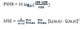
| Step8: Using the below shown equations, MSE and PSNR values are calculated for many RGB test images. | ||||||||||||||||||
 |
||||||||||||||||||
| The above algorithm describes the process of working procedure in proposed method. And also shows the sequencing process performance. The PSNR and MSE values are calculated from original and interpolated reconstructed images using the as shown in the equation (11). |
||||||||||||||||||
EXPERIMENTAL RESULTS |
||||||||||||||||||
| The developed Adaptive filter based color filter array interpolation algorithm is tested for many images. The results are shown for RGB original image of size 768x512 is as shown in Fig.2. Later to the original image, random noise is added to produce the random noisy image. It is as shown in Fig.3 gives information about gray scale image of Fig.2 obtained after removal of red and blue channel color information using the CFAI process. Similar procedure is followed for Fig.3 to get Fig5. |
||||||||||||||||||
| Adaptive filtering is done to Fig .5 to get CFA denoisy image as shown in Fig.6.The R,B and G color channel CFA interpolation process is done to Fig.7 to obtained CFAI reconstructed image as shown in Fig.7. The image in developed method is compared to the et al method [1] reconstructed image, in fig.8 and fig.9. The PSNR values in experimental results are various tested images are tabulated as shown in Table I. From the Table I it is noted that PSNR values in proposed algorithm to the comparison with method [1]. |
||||||||||||||||||
| The tabulated PSNR values shows that comparison of proposed and et al method[1] values of demosaicking methods. The proposed method provides better performance values to the images than previous Edge strength filter based CFA interpolation method. And also in this proposed method obtained better resolution images and lower complexity than previous existing demosaicking methods. This spatially adaptive filter based CFAI method yields visually better results with high PSNR. The Tabulated PSNR values as shown that the comparison of proposed and et al method [1], the developed method provide better performance than before existing methods. |
||||||||||||||||||
CONCLUSION |
||||||||||||||||||
| The proposed adaptive filter is used in interpolation is more effectively at red/blue pixel locations and also diagonal edges in RGB images, than many before existing CFA interpolation algorithms. The proposed adaptive filter is well suited for varying image content and provide better results for high frequency color information. The developed demosaicking algorithm using adaptive filter is more robust in comparison with the previous developed algorithms. The results of proposed method are confirmed that, it has the better performance than previous obtainable methods both in visual image quality and in terms of peak signal-to-noise ratio (PSNR), at a lower computational cost. |
||||||||||||||||||
Tables at a glance |
||||||||||||||||||
|
||||||||||||||||||
Figures at a glance |
||||||||||||||||||
|
||||||||||||||||||
References |
||||||||||||||||||
|


