Combining Beam forming and BSS to improve
Source Separation Performance

R. Ruben Johnson; S. Aishwarya

Combining Beam forming and BSS to improve Source Separation Performance

R. Ruben Johnson¹, S. Aishwarya²

PG Student [Signal Processing], Dept. Of Electrical Engineering, Blekinge Institute of Technology, Sweden 1
PG Student [Signal Processing], Dept. Of Electrical Engineering, Blekinge Institute of Technology, Sweden 2

Related article at Pubmed, Scholar Google

Visit for more related articles at International Journal of Advanced Research in Electrical, Electronics and Instrumentation Engineering

Abstract

Beam forming (BF) and Blind Source Separation (BSS) are always two interesting methodologies to witness in order to separate two sources. BSS in frequency domain have been facing a serious issue of permutation ambiguity while performing source separation using Independent Component Analysis (ICA). Permutation Ambiguity is a problem of mismatch of any frequency lines between the sources, so the separation in the time domain cannot exhibit a perfect separation due to the frequency components of other sources present in the time signal of one source. Various methods have been adopted all through the years of research to get rid of this critical issue and no perfect results are produced so far. The proposed method of combining BF to BSS seems to be a good approach as BF mainly depends on time difference of arrival information (delay) between the reference microphone to the consecutive microphones. The original delay information is compared to the estimated delays for each frequency lines in order to realign the frequency lines if they see a permutation by ICA. So, there is no possibility of frequency mismatch still existing when the delay information is operated as a major concern. The performance is measured using Signal to Interference Ratio measurement where Beamforming approach seems to have an improved performance compared to other existing methods. Simulation results show performance comparison. The algorithm is tested using two speech sources in a free field environment. We use Short Time Fourier Transform (STFT) for frequency domain transformation

Keywords

Blind Source Separation, Beam forming, Independent Component Analysis, Time Difference of Arrival, Signal to Interference Ratio.

INTRODUCTION

Blind Source Separation (BSS) is the process of estimating source signals from the observed signals from any input channel like microphones. Here, the independence of each signal corresponds to the separation of sources.

Similarly, Beamforming is an array signal processing technique which is used to localize sources from different directions. This uses number of linearly arranged microphones. Both these have their own uniqueness and disadvantages as long as they are implemented separately in different applications. Applications like speech enhancement, hearing aids, conference telephony, party gathering, noise-robust speech recognitions and hands-free telecommunication systems requires these processes to have source intelligibility without any irregularities. When BSS is combined with beamforming, it is possible to overcome the drawbacks faced in both the processes. The Beamforming approach is robust since a misalignment at a frequency does not affect other frequencies while in other approaches misalignment may cause consecutive misalignments [1]. Beamforming defines the direction of arrival from Delay and Sum Beamforming algorithm and BSS uses ICA algorithm where both can be made to meet at a common point in order to solve the issue of source separation. This project deals with the point where they both are expected to be combined and the constraints that have to be considered to do this combination.

SURVEY OF RELATED WORKS

Different approaches exist to solve this problem. Basically the permutations can be picked out and frequency band switching is done. The basic idea is to locate the permutations by noticing sudden changes in some properties of the filters or the spectra of the estimated components. In [2] paper, Broadband beamforming with wavelet filter banks were used in the speech enhancement systems to retriever full-band speech signals. In [3] Blind beamforming algorithms were used to recover desired signals without array geometry knowledge. They used multi-stage constant modulus array algorithm to recover the independent signals and also estimate the direction of arrival angles. In [4] paper, they used methods like envelope continuity and filter continuity while using ICA framework to separate sound sources. In [4], null-beamforming based on the direction of arrival was used to optimise and converge ICA algorithm. In our paper, we use a simple Beamforming approach that gives a time difference of arrival estimation which we have used as an apriori information over every frequency lines to separate the mixed sources.

PROBLEM STATEMENT AND MAIN CONTRIBUTION

In a real-time scenario when multiple speakers speak at the same time observed in an array of sensors, the recordings will always contain mixed sources having little or no information about the original sources. It is a very classical and difficult problem to separate them into independent sources. When this problem is investigated in frequency domain, the major issue is Scaling and the Permutation Ambiguity. Our paper focuses on two major research questions:

1. How can Beamforming approach be employed to solve permutation ambiguity in order to improve the efficiency of BSS?

2. How to examine the performance of beamforming approach over inter-frequency dependence methods? Our method proposes to implement Delay and Sum Beamforming in order to solve the issue of permutation ambiguity. Beamformer has the ability to localize the sources using the Time Difference Of Arrival (TDOA) information to the microphone which will be very useful to sort the permutation ambiguity. The TDOA approaches in the previous existing researches were a bit complex while our approach is simple by comparing the estimated time difference with the original time difference and the permuted frequency lines are sorted. Signal to Interference Ratio (SIR) is calculated and compared in-order to examine the performance of Beamforming approach over Inter Frequency Dependence methods. The main contribution in the paper is the implementation of Time Difference of Arrival (TDOA) based approach over existing methods to solve the issue of frequency permutation. For that, Delay and Sum Beamforming is developed for a spherical wave set-up and that delay information is taken as the main attribute to get estimated delays.

PROBLEM SOLUTION

The problem that arise in conference hall, hands-free telecommunication systems, automobiles or in noise-robust speech recognition due to mixed sources requires an appealing solution to separate the mixed sources in each input channel. Beamforming based TDOA approach integrated with this independent source signal vector helps to solve the problem of source separation.

A. Modelling: System modeling is the most important part of any experimental setup. We had a test plan with speech as the sound sources. So the system consists of microphone array having 2 spherical wave sources placed at a suitable height from the array plane. Before we define the system modeling, it is necessary to describe the need for microphone array for the experimentation.

1. Microphone Array

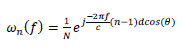
Microphone array is a collection of multiple microphones in a certain arrangement functioning as a unidirectional input device. Here, we consider source as a spherical wave front from the point source which has a different impact on a microphone array. It is because all the applications we aim at are near-field applications which requires array set-up to be closer to the speaker. It considers the radius of the wave to calculate the time delay and the formula is shown below.

(1)

where, is the distance between the source and the microphone array. The array used for our setup is a rectangular array consisting of 8x8 microphones in non-linear fashion. It is arranged in x-y plane where source is placed parallel to this array. Distance between the microphones is set to be 0.0425m, decided depending on the wavelength of the source signal used.

2. Aliasing Effect

It is possible to define the threshold frequency of an equally spaced array as follows,

(2)

Where, is the speed of sound and d is the spacing between the microphones. If the sound source frequency exceeds this critical frequency, ghost sources appear in the beam-pattern [5]. When the sound source frequency is less than the critical value, a main lobe identifies the real emitting source, while the typical side lobes decrease. Exceeding the critical frequency, instead, many ghost sources appear. Thus, the standard solution to avoid aliasing errors is the reduction of the microphone spacing .

(3)

B. Beamforming: Beamforming is the process of performing spatial filtering i.e., the response of the array of sensors is made sensitive to signals coming from a specific direction while signals from other directions are attenuated [6]. Beamformers combine the signals from spatially separated array sensors in such a way that the array output emphasizes signals from a certain “look” direction. Thus if a signal is present in the look-direction, the power of the array output signal is high and if there is no signal in the look-direction the array output power is low.

1. Delay and Sum Beamforming

The delay and sum beamformer is based on the idea where the output signal from each sensor will be the same, except that each value from each sensor will be delayed by a different amount. The radius of the spherical wave-front is defined by,

(4)

where, is the number of microphones in an array and is the distance between the microphones.

The output of each sensor is delayed appropriately and then added together, the response of an array of sensors is made sensitive to signals coming from a specific direction while signals from other directions are attenuated. Usually, each channel is given an equal amplitude weighting in the summation, so that the directivity pattern demonstrates unity gain in the desired direction. This leads to the complex channel weights,

(5)

Expressing the array output as the sum of the weighted channels we obtain

(6)

Equivalently, in the time domain, we have,

(7)

C. Blind Source Separation: Recently, Blind source separation by Independent Component Analysis (ICA) has received attention because of its potential applications in signal processing such as in speech recognition systems, telecommunications and medical signal processing [7]. The goal of ICA is to recover independent sources given only sensor observations that are unknown linear mixtures of the unobserved independent source signals.

1. Independent Component Analysis.

ICA is one of the methods to separate sources from the recordings. As the name indicates, this method separates the mixed recordings into independent components. The recordings and sources are considered as a set of random variables. Therefore here independence has to be taken with its statistical meaning [8]. Two independent variables and are statistically independent if and only if their joint probability density function(pdf) is the product of their marginal pdf.

(8)

Therefore ICA aims at getting as close as possible to this equation. If more than two components are involved, say n, the previous equation is extended to the n-th dimension: the variables are independent

2. Frequency Domain BSS

Different methods have been developed to solve this problem. One is the time domain approach and the other is the frequency domain. [9]. Time domain approach is fairly complicated; require strong computation resources and computation time with the existing algorithms whereas frequency domain approach is known to be faster and easy to apprehend and implement. It is possible to formulate the time domain BSS equation into frequency domain. It is well known that the convolution that appears in time domain equation will be expressed as a simple product in the frequency domain

(9)

The main idea for solving convolutive ICA problems can be seen as the following simplified steps:

Transform the recordings into the frequency domain using Fourier transform

For each frequency, solve the instantaneous mixing case

Pass the independent components found back to the time domain using inverse Fourier transform

Before we go into the processing details, we have to consider the type of mixing used in our algorithm. There is a common assumption of taking instantaneous mixing where the recording is done in linear combination of sources with the real coeffecients, say,

(10)

where, A is a random full rank matrix,

But, in real time, they are not instantaneous anymore but consist of filtered versions of the original sources in each recording. They are called convolutive mixing.

(11)

where, is the impulse response of the environment from the position receiver i to source j. The expression denotes the convolution between the impulse response and the signal originated by source [7].

3. Problems Due to Frequency Domain BSS

The first problem is the problem of conventional Fourier transform. If one recorded signal is changed into frequency domain using a conventional Fourier transform, it will result into one new signal where each sample corresponds to one frequency. Hence all the time-related information is lost and the ICA algorithm derived before will be helpless as it relies on averages of contrast functions over time. Thus we use -Time Fourier Transform (STFT). A short-time Fourier transform of the signal contains information about its frequency content and the variations of this content over time [8]. The most delicate problem and the main issue of BSS in the frequency domain approach is the permutation ambiguity, this ambiguity is induced by the instantaneous ICA algorithm. However in this frequency domain approach, it can be seen that for each frequency a new instantaneous ICA problem has to be solved. So there are as many instantaneous problems to solve for as many frequency bins. But due to the permutation ambiguity, for different frequencies, the components will be evaluated in a priori different order. In order to be reconstructed and transformed back to the time domain, the random permutations have to be targeted and reversed.

4. Fast ICA

The algorithm that will be described in the following is actually the FastICA algorithm developed at Helsinki University of Technology. Many other algorithms exist, however the simplicity and excellent efficiency of the FastICA algorithm made it a good choice to be studied and used here. The algorithm can be seen as two independent parts. First, the data have to be preprocessed and then the optimization part for this preprocessed data. The algorithm will be presented step by step in what follows [8].

a) Pre Processing of Data

To perform ICA we need to preprocess our data. The preprocessing mainly comprises of two steps. Centering the data and Whitening the data. Centering is done to ensure that all the recordings have zero mean and whitening is a simple linear transformation that provides unit variance recordings.

b) Algorithm

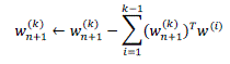
After the data had been pre-processed by means of centering and whitening, the algorithm has to repeat the following process for each vector w.

1. Starting the algorithm with a chosen or a random vector

2. The iteration process starts here and has to be repeated as long as the convergence test at its end fails:

Compute next step using the following equation

Apply basic Gram Schmidt orthogonalization (to force the orthogonality of the un-mixing matrix): if the k-th vector is evaluated and it is the n + 1 step of the iteration, let us use the notation for the vector. Then the orthogonalization is achieved through

Normalize

to force unit variance of the result

Test convergence, for instance by evaluating. If there is any convergence, store the current value f , reset index n to zero, raise index k and go back to step 1 if there are still components to evaluate (k < n). If there is no convergence, continue the iteration process, raise n and go back to step 2.

When k = n, all the components have been evaluated. The independent components are given back by taking each )x, for 1 < k < n.

D. Implementation: A convolutive blind source separation system can be viewed as multiple sets of adaptive beamforming, which means the separation filter array for every output can be viewed as a beamformer. Thus a beamforming approach is used to combine with frequency domain convolutive BSS to deal with frequency permutation problem.

1. Time Difference of Arrival

A convolutive blind source separation system can be viewed as multiple sets of adaptive beamforming, which means the separation filter array for every output can be viewed as a beamformer. The fundamental principle behind DOA estimation using microphone arrays is to use the phase information present in signals picked up by microphones that are spatially separated. Since the sources are spherical it is not necessary to calculate DOA. Instead we go for Time Difference of Arrival (TDOA).

If we have M microphones, we can define − 1) TDOA of a source, for each pair of microphones. Thus, let us consider as below,

(12)

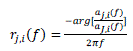
where, r is the original time difference of arrival and (tow) is the time delay between source k to microphone j where J is the reference microphone. Now, while we have original time delay information, it is necessary to find out the estimated time difference of arrival. We have to find the mixing matrix value from the separation matrix W obtained from ICA gives the estimated mixing matrix understood from the formula of IC where mixing matrix and Y is the independent signal which is expected to be similar to the original source signal at ideal conditions. This A gives basis vector elementswhich are used to determine the estimated time difference of arrival. Each basis vector elements in the matrix A is used to calculate TDOA as in the formula,

(13)

where, r is the time difference of signal with respect to microphone. Here, two different subscripts k (original source index) and i (estimated source index) are used for the source index to calculate original TDOA and estimated TDOA because permutation alignment is not done in this stage.

2. Combining Technique

TDOA technique is used as the proposed method here to solve the problem of permutation ambiguity. It is a simple robust technique to align the frequency bins of the independent source signals Y according to the time delay information obtained using TDOA formula [10]. The original TDOA of each pair of microphones is calculated to be that has been calculated using the original time delay information and is used as reference to compare with the estimated TDOA for each frequency bins. The estimated TDOA for each frequency bins gives a value that would be far nearer to any one of the original TDOA corresponding to any source. So, they are compared to see whether the estimated TDOA has a nearer value to either TDOA of source 1 or source 2. So, this is done with all frequency bins Suppose, the TDOA value currently present in 1 seems to have a value nearer to the original TDOA o, the corresponding frequency bin is permuted so as to group the frequency bin of source 1. If there is no such mismatch with1 and or 2 with1, then they are left as such without any alignment. This is continued throughout all frequency bins to check whether they are permuted in anyways. Here, interestingly, the corresponding columns of the separation matrix W are also permuted when the rows of independent source signals1 and2 are permuted. If this is done to all the frequency bins, then they are scaled back to the time domain in order to physically hear to the estimated sources. Now, we could hear a clearly separated speech very much equal to the original speech.

E. Validation: This method is tested on various scenarios of mixed speech signal and analyzed by comparing the results with the previously implemented method (Envelope Continuity). The entire test is operated for two recordings and two sources.

1. Method

A system was modelled with 64 microphones (8X8) and 2 sources. Only free-field condition is considered here. From the microphone array we could easily find the position of the source in space and calculate the time difference of arrival for each microphone. Since just 2 microphones are enough to separate the signals, any 2 adjacent microphones are selected from the array and source separation is performed. For our case we have considered two speech signals of length 4sec and the separation has been carried out. The spectrogram of both the signals is shown in fig.3. Fig.3.

2. Signal to Interference Ratio

Signal to interference ratio (SIR) is a measure of the level of a desired signal to the level of the interfering signal. It is defined as the ratio of the signal power to the interfered signal.

(14)

3. Comparison of TDOA and Envelope Continuity

Various scenarios have been considered as an input to the algorithm, they are discussed as follows

a) Varying the distance between the microphones

First the distance between microphones was changed and the performance was recorded. The graph shows the variation of SIR improvement when the distance between the microphones are changed. SIR improvement of the envelope continuity in this case was not able to follow a trajectory while the SIR improvement of the TDOA method is predictable. Envelope continuity method has a great effect on the initialization vector of the Fast-ICA algorithm as discussed above.

In TDOA the SIR improvement decreases when the distance between microphones increase because the delay will increase when the distance between microphones keep increasing. This may certainly lead to decrease in separation performance as the microphones may not receive sources completely and thus selecting the right source to permute back would be a problem causing the decrease in SIR improvement.

b) Varying the distance between the sources

Secondly the distance between the sources was changed and the performance was recorded, the fig.5. shows that when the distance between the sources increases, there is a decrease in SIR improvement. For both envelope continuity and TDOA, initially in the graph, there is an increase in SIR improvement and then it starts decreasing. The initial increase in the SIR improvement is due to the fact that the sources are in a right position for the system to obtain the maximum SIR improvement. Then, the decrease in SIR improvement is due to the fact that the source signals may not reach the recording system properly. The delays are larger and will be almost the same for both the sources so there is a confusion of aligning the delays of each frequency line to its respected source, thereby creating permuted sources again. But apart from this, the initialization vector in the ICA algorithm plays a major role for this order less trajectory on both the methods. It should have a very good convergence rate of 500 or 1000 depending upon the choice of the initialization vector in order to have a gradual trajectory pattern.

c) Varying the distance between the planes

The third scenario is to change the distance between the microphone array plane and the source plane to check the SIR improvement. As in the previous case, for both envelope continuity and TDOA, there is an initial increase in the SIR improvement in fig.6. is due to the right position for the system to obtain the maximum SIR improvement. Then it gets reduced for the same reason we have discussed above, Initialization vector is the major role for this oscillatory trajectory for both the methods.

d) Varying the filter length

The final scenario is to change the window length for the STFT function. Here in fig.7. for both envelope continuity and TDOA, we could see the drop in SIR improvement when there is an increase in window length for the STFT function. For a little increase in window length for eg. (256 to 512), there is more number of frequency lines at a closer interval, which can form a smooth curve and thus gives a better performance in SIR. But for the further increase in window length such as 1024 or 2048, it results in decrease in the SIR improvement which is due to the less number of computational time signals available when separating the sources apart from having more number of frequency lines at closer interval. Still, when we compare both the methods, TDOA performs better than envelope continuity which is the advantage of the proposed method.

CONCLUSION

In this project, we have reviewed and implemented the approach of combining Beamforming and BSS for convolutive mixtures for a better separation performance. Solving permutation ambiguity was the main aim of this project. We proposed TDOA technique to solve this issue. The algorithm is tested using 2 speech mixtures (male and female voice of 4 sec. audio). Results were evaluated in terms of SIR improvement. Simulation results confirm our expectations and show that TDOA works pretty well than the envelope continuity method in all the conditions. When microphone positions are changed, the performance of TDOA is better and highly predictable compared to envelope continuity. Envelope continuity did not follow a predictable decreasing fashion of SIR and it oscillates for every increase in microphone distance. Similarly, with the increase in the window length, both TDOA and envelope continuity decreases in its SIR improvement. But, for the highest value of window length, the performance of TDOA is very much better than envelope continuity. SIR is better even at the worst case scenario also, for TDOA.

We have implemented this technique in free field simulation. The future work would be to implement this method to the real environment. Since Fast-ICA has a random initialization vector and has a lots of parameters to consider, more robust algorithms like JADE algorithm can be replaced over Fast-ICA

ACKNOWLEDGEMENT

We thank our family, friends in India and Sweden, our professors at Blekinge Tekniska Hogskolan and Bruel &Kjaer Sound and Vibration Measurements A/S, Denmark, whose valuable support and guidance made the successful accomplishment of this project.

Figures at a glance


Figure 1	Figure 2	Figure 3	Figure 4

Figure 5	Figure 6	Figure 7

References

Benny Sällberg, “Applied Methods for Blind Speech Enhancement”, Doctoral Dissertation, Department of Signal Processing, Blekinge Institute of Technology, Sweden 2008.
Dongxia Wang, JiachaoZheng, Tao Wu, “A Broadband Beamforming Method Based on Microphone Array for the Speech Enhancement,” 2010 2nd International Conference on Signal Processing Systems(ICSPS), Jinzhou, 2010, pp.363-366
Ji Zhou, Chao Sun, Yixin Yang, “Experimental Studies on Direction Finding via Blind Beamforming” IEEE, 2010, pp. 281-284
Hiroshi Saruwatari, Toshiya Kawamura, Tsuyoki Nishikawa, Akinobu Lee, KiyohiroShikano, “Blind Source Separation based on a Fast Convergence Algorithm Combining ICA and Beamforming,” IEEE Trans. on Audio, Speech and Language Processing, vol.14, no.2, pp.666- 678, March 2006.
A. Cigada, M. Lurati, F. Ripamonti and M. Vanali, “Beamforming method: Suppression of spatial aliasing using moving arrays,” in BerlinBeamforming Conference, Berlin, 2008.
Grant Hampson and Andrew Paplinski, “Simulation of beamforming techniques for the linear array of transducers”, Department of Robotics and Digital Technology, Monash University, Australia, 1995.
Pierre Comon and Christian Jutten, Handbook of Blind Source Separation: Independent Component Analysis and Applications, 1st edition. Burlington, MA: Elsevier, 2010.
Douglas H, Gupta M, Sawada H and Makino S,”Spatio-temporal FastICA algorithms for the blind separation of convolutive mixtures,” IEETrans. Audio Speech Lang. Process., vol.15, no. 5, Jul., 2007.
Sawada H, Mukai R, Araki S and Makino S, “Convolutive blind source separation for more than two sources in the frequency domain,” in Proceedings of International Conference on Acoustics, Speech and Signal Processing, Montreal, 2004, pp. 885-888.
Shoji Makino, Te-Won Lee and Hiroshi Sawada, Blind Speech Separation. The Netherlands: Springer 2007.