I. INTRODUCTION
|
| This project entitled “Comparative Analysis of advanced Face Recognition Techniques”, it is based on fuzzy c means clustering and associated sub neural network. It deals with the face recognition plays an important role in many applications such as building/store access control, suspect identification, and surveillance. Over the past 30 years, many different facerecognition techniques have been proposed, motivated by the increased number of real-world applications requiring the recognition of human faces. There are several problems that make automatic face recognition a very difficult task. The face image of a person input to a face-recognition system is usually acquired under different conditions from those of the face image of the same person in the database. |
| Therefore, it is important that the automatic face-recognition system be able to cope with numerous variations of images of the same face. The image variations are mostly due to changes in the following parameters: pose, illumination, expression, age, disguise, facial hair, glasses, and background. In many pattern-recognition systems, the statistical approach is frequently used. Neural-network (NN)-based paradigms, as new means of implementing various classifiers based on statistical and structural approaches have been proven to possess many advantages for classification because of their learning ability and good generalization. Generally speaking, multilayered networks (MLNs), usually coupled with the back propagation (BP) algorithm, are most widely used for face recognition. As one drawback of the BP algorithm, when the scale of the NN increases, the computing efficiency decreases rapidly for various reasons, such as the appearance of a local minimum. The HCM is the most well-known conventional (hard) clustering method. The HCM algorithm executes a sharp classification, in which each object is either assigned to a cluster or not. Because the HCM restricts each point of a data set to exactly one cluster and the individuals belonging to each cluster are not overlapped, some similar individuals cannot be assigned to the same cluster, and, hence, they are not learned or recognized in the same NN. In this paper, fuzzy c-means (FCM) is used. In contrast to HCM, the application of fuzzy sets in a Classification function causes the class membership to become a relative one and an object can belong to several clusters at the same time but to different degrees. FCM produces the idea of uncertainty of belonging described by a membership function, and it enables an individual to belong to several networks. Then, all similar patterns can be thoroughly learned and recognized in one NN. |
II. PREPROCESSING
|
Lighting Compensation
|
| We adjusted the locations of the lamps to change the lighting conditions. The total energy of an image is the sum of the squares of the intensity values. The average energy of all the face images in the database is calculated. Then, each face image is normalized to have energy equal to the average energy Energy = Σ (Intensity)2 . |
Facial-Region Extraction
|
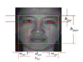
| The method of detecting and extracting the facial features in a grayscale image is divided into two stages. First, the possible human eye regions are detected by testing all the valley regions in an image. A pair of eye candidates is selected by means of the genetic algorithm to form a possible face candidate. In our method, a square block is used to represent the detected face region. Fig. shows an example of a selected face region based on the location of an eye pair. The relationships between the eye pair and the face size are defined as follows |
| hface=1.8deye |
| heye = 1/ε hface |
| weye=0.225 hface |
| Then, the symmetrical measure of the face is calculated. The nose centerline (the perpendicular bisector of the line linking the two eyes) in each facial image is calculated. The difference between the left half and right half from the nose centerline of a face region should be small due to its symmetry. |
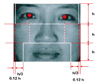
| a threshold value, the face candidate will be selected for further verification. The facial feature regions will exhibit a low value on the projection. A face region is divided into three parts, each of which contains the respective facial features. The projection is the average of ray-level intensities along each row of pixels in a window. In order to reduce the effect of the background in a face region, only the white windows, as shown in Fig. are considered in computing the projections. The top window should contain the eyebrows and the eyes, the middle window should contain the nose, and the bottom window should contain the mouth. |
| This method is called the Linear Discriminant Analysis. Here the low-energy discriminant features of the face are used to classify the images. |
| The transformation matrix W for the LDA is given by the eigenvectors corresponding to the largest eigenvalues of the scatter matrix function (SW--1. SB), where SW is the within-class scatter matrix and SB is the between-class scatter matrix. These scatter matrices are defined as: SB = ΣC Ni (ClasAvgi - AvgFace) (ClasAvgi -AvgFace) T SW = ΣC ΣXi ( xk - ClasAvgi ) ( xk – ClasAvgi )T where, C is the number of distinct classes, Ni is the number of images for each class i, ClasAvgi is the average face image of faces in class i, Xi represents the face images that are in class i, AvgFace is the average face image for all images in the dataset. |
| The steps involved in implementing the algorithm are: Training the Faces: |
| 1. Represent the faces in the database in terms of the vector X . |
| 2. Compute the average face AvgFace and subtract the AvgFace from the vector X. |
| 3. Classify the images based on the number of unique subjects involved. So the number of classes, C, will be the number of subjects who have been imaged. |
| 4. Compute the scatter matrix |
| 5. Use PCA to reduce the dimension of the feature space to N – C. Let the eigenvectors Obtained be WPCA. |
| 6. Project the scatter matrices onto this basis to obtain non-singular scatter matrices SWN and SBN. |
| 7. Compute the generalized eigenvectors of the non-singular scatter matrices SWN and SBN so as to satisfy the equation SB*WLDA = SW*WLDA*D, where D is the eigenvalue. Retain only the C-1 eigenvectors corresponding to the C-1 largest eigenvalues. This gives the basis vector WLDA |
| 8. Then the image vector X is projected onto this basis vector and the weights of the image are computed. |
| Recognition of a new face is done similar to that of the PCA method. Then the Euclidean measure is used as the similarity measure to determine the closest match for the test image with the face in the trained database. |
III.IMPLEMENTATION
|
1. FUZZYC MEANS CLUSTERING:
|
| In fuzzy clustering each point has a degree of belonging to clusters, as in fuzzy logic, rather than belonging completely to just one cluster. For each point x we have a coefficient giving the degree of being in the kth cluster uk(x). Usually, the sum of those coefficients for any given x is defined to be 1: |
 |
| With fuzzy c-means, the centroid of a cluster is the mean of all points, weighted by their degree of belonging to the cluster: |
 |
The degree of belonging is related to the inverse of the distance to the cluster center:  |
| Then the coefficients are normalized and fuzzyfied with a real parameter m > 1 so that their sum is 1. So |
 |
| For m equal to 2, this is equivalent to normalizing the coefficient linearly to make their sum 1. When m is close to 1, then cluster center closest to the point is given much more weight than the others, and the algorithm is similar to k-means. |
| The fuzzy c-means algorithm is very similar to the k-means algorithm: |
| • Choose a number of clusters |
| • Assign randomly to each point coefficients for being in the clusters. |
| Repeat until the algorithm has converged (that is, the coefficients' change between two iterations is no more than ε, the given sensitivity threshold): 1) Compute the centroid for each cluster, using the formula above. 2) For each point, compute its coefficients of being in the clusters, using the formula above. The algorithm minimizes intra-cluster variance as well, but has the same problems as k-means; the minimum is a local minimum, and the results depend on the initial choice of weights. It has better convergence properties and is in general preferred to fuzzy-c-means. |
2. Parallel NNs :
|
| The parallel NNs are composed of three-layer BPNNs. A connected NN with 32 input neurons and six output neurons have been simulated (six individuals are permitted to belong to each subnet). The number of hidden units was selected by six fold cross validation from 6 to 300 units. The algorithm added three nodes to the growing network once. |
| i. Learning Algorithm: A standard pattern (average pattern) is obtained from 12 patterns per registrant. Based on the FCM algorithm, 20 standard patterns are divided into several clusters. Similar patterns in one cluster are entered into one subnet. Then, 12 patterns of a registrant are entered into the input layer of the NN to which the registrant belongs. |
| ii Recognition Algorithm: When a test pattern is input into the parallel NNs, as illustrated in Fig. 5, based on the outputs in each subnet and the similarity values, the final result can be obtained as follows. |
| Step 1. Exclusion by the negation ability of NN. First, all the registrants are regarded as candidates. If the maximum output values are less than the threshold value, corresponding candidates are deleted. The threshold value is set to 0.5, which is determined based on the maximum output value of the patterns of the nonregistrant. |
| Step 2. Exclusion by the negation ability of parallel NNs. Among the candidates remaining after Step 1, the candidate that has been excluded in one subnet will be deleted from other subnets. If all the candidates are excluded in this step, this test pattern is judged as a nonregistrant. |
| Step 3. Judgment by the similarity method. If some candidates remain after Step 2, then, the similarity measure is used for judgment. The similarity value between the patterns of each remaining candidate and the test pattern is calculated. The candidate having the greatest similarity value is regarded as the final answer. |
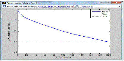
| This paper was analyzed depending upon the time and performance. The face was identified by PCA and LDA method. The table 4.1 shows the result of the performance and time analysis. |
V. CONCLUSION
|
| This project proposed a fuzzy clustering and parallel NNs method for face recognition by using PCA and LDA method. The patterns are divided into several small-scale subnets based on FCM. Due to the negation ability of NN and parallel NNs, some candidates are excluded. The similarities between the remaining candidates and the test patterns are calculated. It judged the candidate with the greatest similarity to be the final answer when the similarity value was above the threshold value. Otherwise, it was judged to be nonregistered. This project was compared with LDA and PCA method, and it was analyzed .The result of this analysis is, the PCA method is better than the LDA. |
Tables at a glance
|
 |
 |
| Table 1 |
Table 2 |
|
| |
Figures at a glance
|
 |
 |
 |
| Figure 1 |
Figure 2 |
Figure 3 |
|
| |
References
|
- A. Z. Kouzani, F. He, and K. Sammut, “Towards invariant face recognition,”Inf. Sci., vol. 123, pp. 75–101, 2000.
- K. Lam and H. Yan, “An analytic-to-holistic approach for face recognition based on a single frontal view,” IEEE Trans. Pattern Anal. Mach.Intell. vol. 20, no. 7, pp. 673–686, Jul. 1998.
- P. J. Phillips, “Matching pursuit filters applied to face identification,”IEEE Trans. Image Process., vol. 7, no. 8, pp.1150–1164, Aug. 1998.
- M. A. Turk and A. P. Pentland, “Eigenfaces for recognition,” J. Cognitive Neurosci., vol. 3, pp. 71–86, 1991.
- T.Yahagi and H. Takano, “Face recognition using neural networks with multiple combinations of categories,” J. Inst. Electron. Inf. Commun.Eng., vol. J77-D-II, no. 11, pp. 2151–2159, 1994, (in Japanese).
|