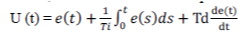
We designate PID (Proportional Integral Derivative) controller in industries for various process control applications. It provides control action to the discrepant values from the desired values in process output. CSTR (Continuous Stirred Tank Reactor) is the most important process which plays a significant role in process and chemical industries. We have to control various process variables like temperature, concentration, flow, pressure etc. in this process. Hence we need appropriate control action to maintain this process in the desired condition. We use PID controller which yields an overshoot and long settling time, which exacerbate the process. Hence it is not well suited for many complex processes in industries. So we are going for a better type of controller, known as MPC (Model Predictive Control). It is very accurate and reliable in controlling the process variable. MPC has the ability to anticipate the future events and takes action accordingly. In this manuscript comparison of PID controller with MPC is made and we examine the best controller for this CSTR temperature control process.
Keywords |
| Continuous Stirred Tank Reactor, MPC controller, PID controller, CSTR temperature control process. |
INTRODUCTION |
| Normally CSTR process is very complicated in nature and deals with multiple aspects in industries [1]. It consists of
more than one process variables and manipulated variables. All the variables in this process are correlated. Any
changes in the single variable lead the system to undesirable behaviour [4]. We have to control all the variables based on
their relationship between them for controlling the system in a desired value. In industries, they use cascade controller
for getting more accurate control action for this process [6]. PID controller plays a crucial role in industries [2]. Due to its
demerits we are going for new type of controllers. |
| Designing a controller to this process is very complicated and big challenge for engineers [10]. Many process and
chemical industries uses this CSTR process. There they have to use lots of controller for maintaining the process in
desired condition. So we need to use more than one sensor for measuring each parameter from this process. The
measured physical variable in this process can be used for designing the controller [8]. In this paper, we are going to find
out which controller is going to give an appropriate control action for this CSTR temperature control process. By
comparing the controllers one with another, we can finalise the result based on the performance index and time domain
specifications [3]. Every controller behaves on its own way in maintaining the process into a desired value. |
| In the previous paper, they told that we get good performance for the CSTR temperature control process using 2 DOF
PID [2]. They are using 2DOF PID controller for this process. It gives satisfactory result to the engineers. In another
paper they told that they are getting better solution for the CSTR temperature control process by using polymath
programming [3]. They finalised the result using this polymath programming method. |
CSTR PROCESS |
| Continuous stirred tank reactor (CSTR) is a one which is used in various chemical and process industries [3]. It
is also called as vat or back mix reactor [5]. The reactants are continuously fed into the reactor. The reactant is mixed
perfectly for getting product in chemical industries. For getting perfect reaction by this process, we must control all the
process parameters in desired values [6]. |
| We are going to derive the mathematical model of the CSTR temperature control process. Here the reactor
surrounded by a jacket with coolant with lower temperature than reactor, which is used to diminish the temperature of
the reactor [1]. The flow of coolant around the jacket determines the process temperature. Here controlled variable is
temperature of process and only manipulated variable is flow of coolant in the jacket. |
PROCESS PARAMETER |
| All the systems are identified based upon their behaviour of various dynamic inputs applied to it. The
dynamic behaviour of the system for various inputs is known as SI (System Identification). From the true behaviour of
the system for various inputs, we can derive the mathematical model of the system [7]. For deriving the mathematical
model of the system, first we have to choose process variable from the process and then we need to write mass and
energy balance equation from the given setup. Mathematical model theoretically represents the behaviour of the system
for different inputs. It helps us to steady about the behaviour of the system theoretically before implementing it [9].
Engineers design the controller for the system by using its mathematical modelling. Another way of finding system
behaviour is pragmatic designing [7]. We get the behaviour of the system by designing the system pragmatically. As per
our anticipation about the process response for various inputs using mathematical modelling, we get the same desired
response for implementation of the process pragmatically for the same inputs [8]. This process consists of more than one
process variable. So it is a second order system, the basic second order equation is, |
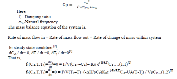 |
 |
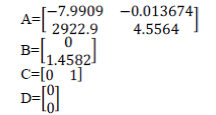
| Reactor parameter’s value:[1] |
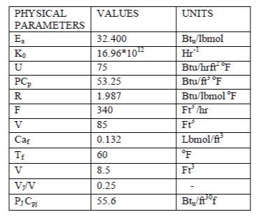 |
| These are all the values taken from the model of the CSTR temperature control process. By substituting these values in
general equation we get the resultant equation from the above derivation in the form of state model [1], |
 |
| By using state space model to transfer function conversion statement in MATLAB, we get the transfer function [t / tf]
of this process [1]. |
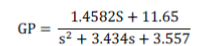 |
| This is the mathematical model of our CSTR temperature control process, which has been derived from the pragmatic
modelled system. |
CONTROLLER DESIGNING |
| A.PID CONTROLLER: |
| Simulation of the CSTR temperature control process has been done by using its mathematical modelling
in MATLAB. The image of the simulated block diagram of the CSTR temperature control process consists of step
input, PID controller, system and scope for visualize the output response. |
| The designing of control parameters for this process is done by various methods. For designing the controller
we need to know about the system response. We apply Astrom and Hagglund relay feedback logic to find the system
response [1]. We have to replace the PID controller with relay for finding the Kp and Pu. |
| We find the Kp and Pu values by using this relay feedback logic in MATLAB for tuning the controller. |
| This figure 1.3 represents the model of for Astrom and Hagglund relay feedback logic. Here the relay is
used for maintain the process variable in the set point. It will hold until the process variable reaches its set value. After
exceeding the desired value it switches the process variable to its negative set value and begins to hold its activity. This
process repeats continuously for a long time in the same interval. Whenever there is a small error in the system or the
output lags input by π radians, the system will start to oscillate with period of Pu. |
| Figure 1.4 shows that how to get the Kp and Pu values from the response curve. Here ‘a’ is amplitude of process
response curve, Pu is a period of process variable oscillations and h is magnitude of manipulating variable. We take
the Ku and Pu values from the response curve. The period of oscillation is 2 sec and gain is 1.4. By using these values
we design the controller. |
| Ziegler-Nichols Tuning method: |
| This method is a trial and error tuning method based on sustained oscillations which was first proposed by Ziegler and
Nichols (1942). This is probably the most widely used method for tuning of PID controller and is also known as online
or continuous cycling or ultimate gain tuning method. Having the ultimate gain and frequency (Ku and Pu) and using
table 1.1, the controller parameters can be obtained. |
| By using this formula, we can find the control parameter. Put this values in general controller equation. |
 |
| After substituting these values in equation, we simulate the process in MATLAB. It gives the response to the discrepant
values of the given CSTR temperature control process. |
| Chien-Hrones-Reswick Auto tuning Method: |
| It is another method of designing a PID controller. It is an efficient method and is used to get the precise control action
to error value. It has four types of formula for designing a controller. By knowing the value of dead time and time
constant we calculate the controller parameters.
The following tables show the Chien-Hrones-Reswick recommendations for each tuning formula: |
| Where TP is the time constant and is the dead time. |
| Where TP is the time constant and is the dead time. |
| Where TP is the time constant and is the dead time. |
| Where TP is the time constant and is the dead time |
| After substituting the controller parameter values in the general equation, we have simulated the setup. |
| Tyreus-Luyben Tuning Chart:The Tyreus-Luyben procedure is quite similar to the Ziegler-Nichols method but the final controller settings are
different. Also these methods only propose settings for PI and PID controllers. These settings are based on ultimate
gain and period is given in the table 1.6. |
| After finding the controller parameter, we substitute those values into the general equation, then simulate the process in
the MATLAB which gives us the response curve. |
| From the above strategy we finalised the best controller for our process. But we already know that, PID controller has
overshoot and long settling time.Hence now we are going for new type of digitalised controller, known as MPC (Modern Predictive Control). |
| B. Model Predictive Control: |
| Modern predictive control is a digital control which is used in chemical and process industries for solving complicated
processes since 1980’s. It needs process parameters to control the process in desired value, which has been obtained
pragmatically by modelling the process. It keeps future time slots into an account and allows the current time slot to be
optimized. MPC can anticipate future events and takes control actions accordingly. But PID controllers and others
cannot predict the future events. |
| Model Predictive Control (MPC) is a multivariable control algorithm that uses: |
| an internal dynamic model of the process |
| a history of past control moves and |
| an optimization cost function J over the receding prediction horizon, |
| The optimization cost function is given by: |
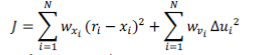 |
| th controlled variable (e.g. measured temperature |
| th reference variable (e.g. required temperature) |
| th manipulated variable (e.g. control valve) |
| weighting coefficient reflecting the relative importance of |
| weighting coefficient penalizing relative big changes in |
| This is the block diagram of modern predictive controller used in MATLAB for simulating the mathematical model of
the process. We configure MPC depends upon the process parameters. It gives as a satisfactory control action to the
process compared with conventional controller. MPC has better control ability over the deviation of the process
variable. |
RESULTS AND DISCUSSIONS |
| From the above controller designing method, we got various types of response for each controller. These
responses provide us a sufficient knowledge about the response of the system for different controller. We tabulated the
time domain specifications and performance index values below. |
| TIME DOMAIN SPECIFICATIONS: |
| Above table1.7 shows the performance of the different controller action upon our CSTR process. Different
controller has different settling time and overshoot. From these results we find out which controller will be best for our
process. From these values we find that Z-N based PID controller is well suited for our CSTR process among the
conventional controller. But we are considering the model predictive controller, it will be the best one for our process.
It has short settling time and lower overshoot percentage. |
| PERFORMANCE INDICES: |
| In this time domain specification and performance criteria, we select the best controller by considering the minor
overshoot and settling time into an account. The comparative analyses of diverse controllers are shown in below figure.
This performance index gives as the possibilities of error during the process for different controller. Minimum ISE and
ITAE value gives the better controller action for the process. |
| Comparison chart has different controller performance and its step response. From this chart we identified that MPC
controller has better performance over our process. Compared with other conventional controller, MPC has minimum
overshoot and settling time. |
CONCLUSION |
| From the above discussion, we identified the best controller for CSTR temperature control process to be MPC. For
controlling temperature in a constant value it is very complicated in industries. MPC controller leverages these
difficulties by bringing the process variable to the desired set point as quickly as possible. Even though MPC controller
is not suitable for a simple system, it is good for a complicated system like our CSTR temperature control processes.
MPC controller has a 0% overshoot and minimum settling time as compared with other conventional controller that we
used in this process. So we can consolidate the performance of all of these responses and we finalised the result as
MPC is the best controller for our CSTR temperature control process. |
Tables at a glance |
 |
|
|
|
|
| Table 1 |
Table 2 |
Table 3 |
Table 4 |
Table 5 |
|
|
|
| Table 6 |
Table 7 |
Table 8 |
|
| |
Figures at a glance |
 |
 |
 |
 |
 |
| Figure 1 |
Figure 2 |
Figure 3 |
Figure 4 |
Figure 5 |
|
| |
References |
- Cheniminekikishore, T.Vandhana, Sheereenhussain and S.Srinivasuluraju,âÃâ¬ÃÂimplementation of model predictive control and auto tuning based PID for effective temperature control in CSTRâÃâ¬ÃÂ, graduate research in engineering and technology,vol.1, no.1, pp.84-89,2012
- Sandeep Kumar, âÃâ¬ÃÂtemperature control of CSTR and PID and PID (Two Degree of Freedom) Controller, international journal of advanced research in computer science and software engineering,vol.2, No.4, pp. 326-329, 2012
- Kansenitin.g, dhankep.b and thombareabhijit ,âÃâ¬Ã modeling and simulation of the CSTR for complex reaction by using polymathâÃâ¬ÃÂ, Research Journal of Chemical Sciences, Vol. 2, No.4 , pp. 79-85, April 2012.
- Astrom K,J, T. Hagllund; âÃâ¬ÃÂPID controllers Theory, Design and Tuning âÃâ¬ÃÂ,2nd edition, Instrument Society of America, pp.1-12, 1994
- Mituhiko and hidefumitaguchi, âÃâ¬ÃÂtwo degree of freedom PID controllerâÃâ¬ÃÂ, international journal of control, automation and systems, vol.1, No.4, pp. 401- 411, Dec 2003
- MohdFuaâÃâ¬Ãâ¢adRahmat,amirmehdiyazdani, mohammadahmadimovahad and somaiyehmahmoudzadeh,âÃâ¬ÃÂtemperature control of a continuous stirrer tank reactor by means of two different intelligent strategiesâÃâ¬ÃÂ, international journal on smart sensing and intelligent system,vol.4, No.2, pp. 244-261, June 2011
- A.D.Shakibjoo, âÃâ¬ÃÂA Comparison of different control design methods for the linearized CSTR temperature modelâÃâ¬ÃÂ, journal of electrical and computer engineering innovations, vol.1, No.2, pp. 107-114, 2013.
- BikashDey, LusikaRoy,âÃâ¬ÃÂA comparative study in temperature control of CSTR using PI controller, PID controller and PID controller(Two Degree of Freedom) controllerâÃâ¬ÃÂ, international journal of electronics and computer science engineering, vol. 3, no.1, pp. 62-68, 2012
- A.Soukkou, A.Khellaf, S.Leulmi and K.Boudeghdegh,âÃâ¬Ã optimal control of a processâÃâ¬ÃÂ, Brazilian journal of chemical engineering, vol.25 No.4, pp. 104- 120, Oct/Dec 2008.
|