ISSN ONLINE(2278-8875) PRINT (2320-3765)
ISSN ONLINE(2278-8875) PRINT (2320-3765)
Prof.Laila Beebi M1, Naveen N S2,Vishakh K H3
|
| Related article at Pubmed, Scholar Google |
Visit for more related articles at International Journal of Advanced Research in Electrical, Electronics and Instrumentation Engineering
Thispaper presents a model-based fault detection system using kalman filter as state estimator. It focuses on the various sensor faults occurring in the RLV. A multiple model adaptive estimator using a bank of kalman filter is used here to model the various faults occurring that are applicable to aerospace systems..
Keywords |
||||||
| fault detection, extended kalman filter, unscented kalman filter, multiple model, residue, RLV. | ||||||
INTRODUCTION |
||||||
| Reusable Launch Vehicles, or RLV's, are space vehicles designed to perform multiple space missions thus dramatically reducing the cost. No true orbital reusable launch system is currently in use. The closest example was the partially reusable Space Shuttle. The development and control of the Reusable Launch Vehicle is one of the major researches going on today. Aerodynamic fault estimation is an integral part of aerospace system design. Sophisticated flight control systems are required for high performance aircraft with instabilities, since the instabilities are beyond the capabilities of human pilot to counteract. | ||||||
| On-line fault estimation techniques such as reconfigurable or adaptive control, system health monitoring, and fault tolerant control etc. are used enabled by the recent advances in computational power. An efficient online fault detection technique is essential for the design of a fault tolerant control system. This paper deals with fault detection technique using a bank of kalman filters. The problem under consideration is the estimation of sensor faults occurring in the RLV in its descent phase.Model-based fault diagnosis method is applied in this work. | ||||||
METHODOLOGY |
||||||
| The process noise and measurement noise in the system are considered as Gaussian white noise with zero mean. Gaussian noise is the random noise appearing in the system whose probability density function is equal to that of the normal distribution. In applications, it is most commonly used as additive white Gaussian noise. | ||||||
| Kalman filter is a commonly used algorithm for recursive parameter identification due to its excellent filtering properties. Failures are caused on the system due to the effects of inaccurate control surface and fail in the flight control system and other faults. | ||||||
SYSTEM DESIGN |
||||||
| Fault-tolerance is the property that enables a system to continue operating properly in the case of occurrence of one or more faults in some of its components. Even a small failure can cause total breakdown in a naivelydesigned system. Fault-tolerance is particularly sought-after in high-availability or life-critical systems like RLV, spacecraft etc. The whole process of fault detection depends on the model used to represent the dynamic system. Better the model better will be the performance of the fault detection scheme and less will be the rate of false alarms. | ||||||
| A reusable launch system (or reusable launch vehicle, RLV) is a launch system which is capable of launching a launch vehicle into space more than once. Aerospace systems are characterized by nonlinear models as well as noisy and biased sensor measurements. An accurate model of the RLV is required to provide the necessary flight control compensation and performance by flight control systems. | ||||||
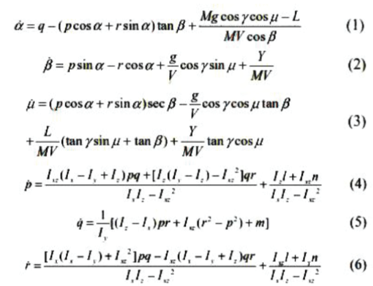
| The nonlinear rigid body attitude motion dynamics of an RLV of dry mass M are modeled by a very complicated set of six non-linear coupled differential equations. | ||||||
 |
||||||
| These states, governed by equations (1-3), are angle of attack (α), sideslip angle (β), and bank angle (μ). Command of these three angles is given by RLV guidance system. Compared to the angle rate dynamics governed by equation (4- 6), the angle dynamics (1-3) are thought of slow dynamics which use the angle rate as control inputs. Equations (4-6) govern the fast states, which include the body axis roll, pitch and yaw rates (p , q and r , respectively). These states are fast in the sense that the control inputs have a significant direct effect on their rates. In the above equations, gdenotes the local gravitational acceleration; L and Y denote the aerodynamic lift and side forces; l,m and n denote the aerodynamic rolling, pitching and yawing moments. The moments of inertia of the symmetric missile are denoted byIi, where i=x, y or z, and its single nonzero product of inertia is represented by Ixz.[6] | ||||||
| These complex set of equations can be decoupled and linearized into the longitudinal and lateral equations under certain assumptions. In this paper the longitudinal dynamics of the RLV in its descent phase is considered. | ||||||
| State equation | ||||||
| wprocess noise with covariance matrix Q. Measurement equation | ||||||
| v measurement noise with covariance matrix R. | ||||||
A. Kalman filter |
||||||
| The Kalman filter, also known as linear quadratic estimation (LQE), is an algorithm that uses a series of measurements observed over time, containing random noise and other inaccuracies, and produces estimates of variables. The algorithm works in a two-step process: in the prediction step, the Kalman filter produces estimates of the current state variables, along with their uncertainties. Once the outcome of the next measurement is observed, these estimates are updated using a weighted average, with more weight being given to estimates with higher certainty. Because of the algorithm’s recursive nature, it can run in real time using only the present input measurements and the previously calculated state; noadditional past information is required. | ||||||
| The Kalman filter model assumes the true state at time k is evolved from the state at (k−1) according to | ||||||
 |
||||||
| WhereA is the state transition model which is applied to the previous state xt|t;B is the control-input model which is applied to the control vector ut; wt is the process noise which is assumed to be drawn from a zeromeanmultivariate normaldistribution with covariance Q. In discrete domain | ||||||
| At time k an observation (or measurement) zk of the true state xk is made according to | ||||||
 |
||||||
| Where C is the observation model which maps the true state space into the observed space and vt is the observation noise which is assumed to be zero mean Gaussian white noise with covariance R. In discrete domain | ||||||
| Prediction state | ||||||
 |
||||||
| Correction state | ||||||
 |
||||||
| It can be seen that if the measurement noise is large, R will be large and thus kalman gain K will be small. So in case of large measurement errors, not much significance is there fo the measurement Y. In case of small measurement errors, R will be small and K will be large and so the measurement Y will be credible for calculating the next state. | ||||||
| Getting a good estimate of the noise covariance matrices Qk and Rkis often difficult. Research has been done to estimate thiscovariance from data. One of the more promising approaches to do this is the Auto-covariance Least- Squares (ALS) technique that uses auto-covariance of routine operating data to estimate the covariance.The kalman filter minimizes the average estimation error thus producing a better estimate. | ||||||
B. Extended Kalman filter |
||||||
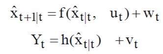
| In the extended Kalman filter (EKF), the state transition and observation models need not be linear functions of the state but may instead be non-linear functions. These functions are ofdifferentiable type. | ||||||
 |
||||||
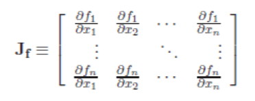
| The function f can be used to compute the predicted state from the previous estimate and similarly the function h can be used to compute the predicted measurement from the predicted state. However, f and h cannot be applied to the covariance directly. Instead a matrix of partial derivatives (the Jacobian) is computed. | ||||||
 |
||||||
| Prediction state | ||||||
 |
||||||
| Correction state | ||||||
 |
||||||
| At each time step the Jacobian is evaluated with current predicted states. These matrices can be used in the Kalman filter equations. This process essentially linearizes the non-linear function around the current estimate. | ||||||
C. Unscented Kalman Filter |
||||||
| When the state transition and observation models, that is the predict and update functions fand h are highly nonlinear, the extended Kalman filter can give particularly poor performance. This is because the covariance is propagated through linearization of the underlying non-linear model. The unscented Kalman filter (UKF) uses a deterministic sampling technique known as the unscented transform to pick a minimal set of sample points (called sigma points) around the mean. These sigma points are then propagated through the non-linear functions, from which the mean and covariance of the estimate are then recovered. The result is a filter which more accurately captures the true mean and covariance. In addition, this technique removes the requirement to explicitly calculate Jacobians, which for complex functions can be a difficult task in itself. | ||||||
Prediction state |
||||||
| As with the EKF, the UKF prediction can be used independently from the UKF update, in combination with a linear (or indeed EKF) update, or vice versa.The estimated state and covariance are augmented with the mean and covariance of the process noise. | ||||||
 |
||||||
| A set of 2L+1 sigma points is derived from the augmented state and covariance where L is the dimension of the augmented state. | ||||||
 |
||||||
| The matrix square root should be calculated using Cholesky decomposition to choose a set of so-called sigma points. The Kalman filter tracks the average state of a system as a vector x of length N and covariance as an N-by-N matrix P. The matrix P is always positive semi-definite, and can be decomposed into LLT. The columns of L can be added and subtracted from the mean x to form a set of 2N vectors called sigma points. These sigma points completely capture the mean and covariance of the system state. | ||||||
| The sigma points are propagated through the transition function fto give transformed sigma points. | ||||||
 |
||||||
| The weighted sigma points are recombined to produce the predicted state and covariance. | ||||||
 |
||||||
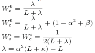
| `where the weights for the state and covariance are given by: | ||||||
 |
||||||
| Typical values for α, β, and κ are 10 − 3, 2 and 0 respectively. (These values should suffice for most purposes.) | ||||||
Correction state |
||||||
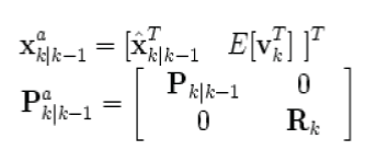
| The predicted state and covariance are augmented as before, except now with the mean and covariance of the measurement noise. | ||||||
 |
||||||
| As before, a set of 2L + 1 sigma points is derived from the augmented state and covariance where L is the dimension of the augmented state. | ||||||
| Alternatively if the UKF prediction has been used the sigma points themselves can be augmented along the following lines. | ||||||
 |
||||||
| The sigma points are projected through the observation function h. | ||||||
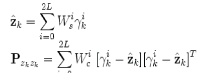
| The weighted sigma points are recombined to produce the predicted measurement and predicted measurement covariance. | ||||||
 |
||||||
| The state-measurement cross-covariance matrix, | ||||||
 |
||||||
| is used to compute the UKF Kalman gain. | ||||||
| As with the Kalman filter, the updated state is the predicted state plus the innovation weighted by the Kalman gain, | ||||||
| And the updated covariance is the predicted covariance, minus the predicted measurement covariance, weighted by the Kalman gain. | ||||||
SIMULATION |
||||||
| In order to compare and validate the estimation schemes, simulations for a RLV during reentry are presented. MATLAB is used for simulation purposes. Mat lab coding is done for both the extended and the unscented kalman filters.The nonlinear system considered here is the dynamics of an RLV in its reentry phase. | ||||||
| A nominal flight condition at an altitude of 30,000 ft. at a Mach number of 0.6 is considered here Process noise covariance and Sensor noise covariance are taken as Q = 1 and R = 2 respectively. The simulation dynamic steps taken are 100. | ||||||
CONCLUSIONS |
||||||
| Kalman filter is used in real time for state estimation. It use stateXt|t’s as optimal estimate of state at time t, and use Pt|t as a measure of uncertainty. Combined with MMAE approach, it’s been able to detect faults in the system in real time. Selecting of threshold band is of great Importance. If threshold is raised to reduce false alarms, time taken for the detection of false also increases. But in fault-critical system such as RLV, this may cause total failure and so a lesser threshold is selected. | ||||||
| In EKF the state distribution is propagated analytically through the first-order linearization of thenonlinear system. It does not take into account that xtis a random variable with inherent uncertaintyand it requires that the first two terms of the Taylor series to dominate the remaining terms.Second-Order version exists, but the computational complexity required makes it unfeasiblefor practical usage. So linearization error problem is amajor problem in extended kalman filter. | ||||||
| Unscented kalman filter approximates the distribution around sigma points and so is accurate to at least the 2nd order.No Jacobians or Hessian are calculated. The UKF consistently achieves a better level of accuracy than the EKF at a comparable level of complexity. | ||||||
Tables at a glance |
||||||
|
||||||
Figures at a glance |
||||||
|
||||||
References |
||||||
|