Boikanyo Makubate1*, Broderick Oluyede2, and Galetlhakanelwe Motsewabagale3
1Botswana International University of Science and Technology Palapye, Botswana
2Georgia Southern University, USA
3Galetlhakanelwe Motsewabagale, Botswana International University of Science and Technology, Botswana
Received date: 08/01/2019 Accepted date: 06/02/2019 Published date: 18/02/2019
Visit for more related articles at Research & Reviews: Journal of Statistics and Mathematical Sciences
We present a new class of distributions called the Dagum-Power Series (DPS) distribution. This model is obtained by compounding Dagum distribution with the power series distribution. Statistical properties of the DPS distribution are obtained. Methods of finding estimators including maximum likelihood estimation will be discussed. A simulation study is carried out for the special case of Dagum-Poisson distribution to assess the performance of the DPS distribution. Finally, we apply the special case of Dagum geometric and Dagum Poisson in the class of (DPS) distributions to real data sets to illustrate the usefulness and applicability of the distributions.
Dagum distribution, Dagum power series distribution, Dagum poisson distribution, Dagum geometric distribution, Dagum logarithmic distribution
Dagum distribution [1,2] is a well-known and established three-parameters distribution for modeling empirical income and wealth data, that could accommodate both heavy tails in empirical income and wealth distributions, and also permit interior mode. A random variable X following the Dagum distribution with shape parameters β, δ>0 and scale parameter λ>0 has a Cumulative Distribution Function (CDF) given by:
 (1)
(1)
The rth raw or non central moments of Dagum distribution are given by:
The rth raw or non central moments of Dagum distribution are given by:
 (2)
(2)
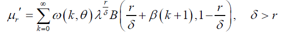
for δ>r, and β,δ>0, where B(.,.) is the beta function. The qth percentile of the Dagum distribution is
 (3)
(3)
Dagum distribution has positive asymmetry, and its hazard rate can be monotonically decreasing, upside-down bathtub and bathtub followed by upsidedown bathtub [3], thus overcoming the forms presented by the exponential, gamma and Rayleigh distributions for modeling lifetime data. Dagum distribution has been used in several research areas such as economics and lifetime data. However, in order to fit still more complex situations, a number of extensions have been proposed in recent years. For example, see the works by Domma, Huang Oluyede [4,7] . It is the purpose of this article to propose a new extension of the Dagum distribution by compounding the Dagum distribution and the power series distributions. The general class is called the Dagum Power Series (DPS) family. We employ the compounding procedure in [8]. The power series family of distributions includes binomial, Poisson, geometric and logarithmic distributions [9]. In the same way, several classes of distributions were proposed by compounding some useful lifetime and power series distributions [10-16]. Also, a primary motivation for the development of this distribution is the modeling of lifetime data with a diverse model that takes into consideration not only shape, and scale but also skewness, kurtosis and tail variation. Also, motivated by various applications of geometric, Poisson and Dagum distributions in several areas including reliability, finance and actuarial sciences, as well as economics, where Dagum distribution plays an important role in the size distribution of personal income, we construct and develop the statistical properties of this new class of generalized Dagum-type distribution called the Dagum-geometric and Dagum-Poisson distributions and apply the models to real life data in order to demonstrate the usefulness of the proposed class of distributions. In this regard, we present the special cases of the compound new four-parameter distributions, referred to as the Dagum-geometric (DG) and Dagum-Poisson (DP) distributions. This paper is organized as follows. In Section 2; we introduce the new family and present a useful representation for its CDF and pdf: We discuss in Section 3 four special models of the proposed family. In Section 4 we present a representation for the hazard and reverse hazard function for the new family.
Some statistical properties of the new distribution including the quantile function, moments, and conditional moments are presented in Section 5. Mean and median deviations, Bonferroni and Lorenz curves are derived in Section 6: The distribution of order statistics and R_enyi entropy are given in Section 7: Maximum likelihood estimates of the unknown parameters are presented in section 8: The special cases of the Dagum-geometric and Dagum-Poisson distributions are discussed in section 9: A simulation study is conducted in order to examine the bias, mean square error of the maximum likelihood estimators and width of the con_dence interval for each parameter of the DP model in section 9: Section 10 contains concluding remarks.
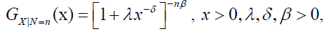
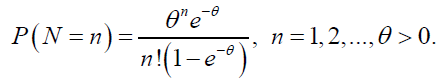
Recently, Dagum distribution has been studied from a reliability point of view and used to analyze survival data [4,17]. Huang and Oluyede [17] developed the exponentiated Kumaraswamy-Dagum distribution and applied it to income and lifetime data. Kleiber [18] provided a comprehensive summary of Dagum distribution. See Kleiber and Kotz [19] for additional results on statistical size distribution with applications in economics and actuarial sciences. Suppose that the random variable X has the Dagum distribution where its CDF is given in equation (1). Given N; let X1,…,XN be independent and identically distributed random variables from Dagum distribution. Let N be a discrete random variable with a power series distribution (truncated at zero) and Probability Mass Function (PMF)
where an ≥ 0 depends only on n,  and θ ÃÆÃÂÃâââ¬Å¾ (0,s) (s can be ∞) is chosen such that C(θ) is finite and its three derivatives with respect to _ are defined and given by C’(.),C”(.) and C’”(.), respectively. The power series family of distributions includes binomial, Poisson, geometric and logarithmic distributions. See Table 1 for some useful quantities including an, C(θ), C(θ)-1, C’(θ); and C”(θ) for the Poisson, geometric, logarithmic and binomial distributions.
| Distribution | C(θ) | C’(θ) | C”(θ) | C(θ)-1 | an | Parameter space |
|---|---|---|---|---|---|---|
| Poisson | eθ -1 | eθ | eθ | Log (1+θ) | (n!)-1 | (0,∞) |
| Geometric | Θ (1-θ)-1 | (1-θ)-2 | 2 (1-θ)-3 | θ(1+θ)-1 | 1 | (0,1) |
| Logarithmic | -log (1-θ) | (1-θ)-1 | (1-θ)-2 | 1- eθ | n-1 | (0,1) |
| Binomial | (1+θ)m-1 | m(1+θ)m-1 | m(m-1)(1+θ)m-2 | (1+θ)1/m-1 |  |
(0,1) |
Table 1. Useful quantities for some power series distributions.
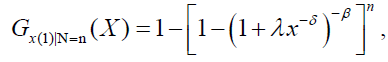
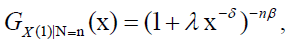
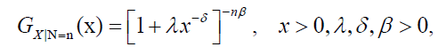
Let X=max(X1,….,XN), then the cumulative distribution function (CDF) of X|N=n is given by:
 (4)
(4)
which is the Dagum distribution with parameters λ, δ and nβ. The Dagum Power series class of distributions denoted is defined by the marginal CDF of X.
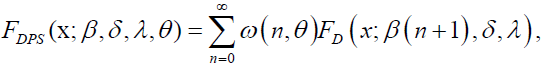
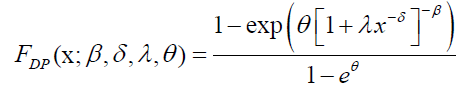
The general form of the CDF and pdf of the Dagum-power series distribution are given by:
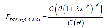 (5)
(5)
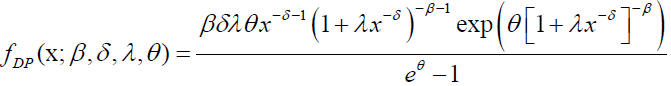
and
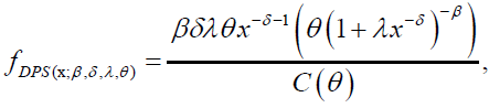 (6)
(6)
respectively, where  with an>0 depends only on n. A series representation of the DPS CDF is given by:'
 (7)
(7)
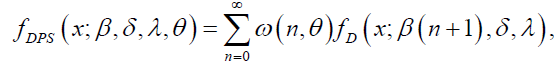
Where 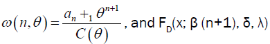 is the Dagum CDF with parameters β (n+1), δ, λ>0. Similarly, the DPS PDF can be written as:
 (8)
(8)
where fD(x, β (n+1), δ, λ) is the Dagum pdf with parameters β (n+1), δ, λ> 0.
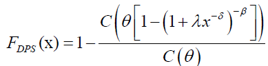
On the other hand, if we consider X(1)=min(X1,…..,XN) and conditioning upon N=n, then the conditional distribution of X(1) given N=n is obtained as:

The CDF of X(1), say FDPS, is given by:
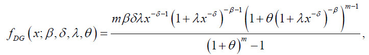
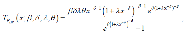
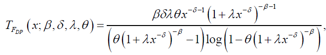
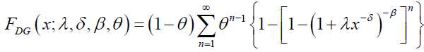
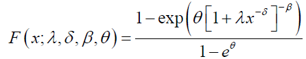
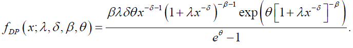
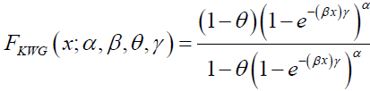
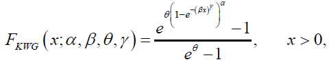
In this section, we present four special cases of the DPS family, namely the Dagum Poisson (DP); Dagum Geometric (DG); Dagum Logarithmic (DL) and Dagum Binomial (DB): For x>0, λ, β, δ, θ>0; the CDF of the DP is defined by equation (5) with C(θ)=eθ-1 leading to:
 (9)
(9)
The PDF of the DP distribution is given by:
 (10)
(10)
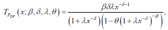
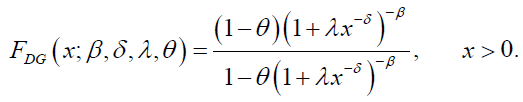
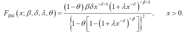
Similarly, the CDF and PDF of the DG distribution are respectively, given by:
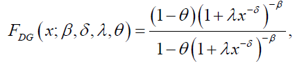 (11)
(11)
and
 (12)
(12)
Whereas, the CDF and pdf of the DL distribution are given by:
 (13)
(13)
and
 (14)
(14)
respectively. Finally, the CDF and PDF of the DB distribution are given by:
 (15)
(15)
and
 (16)
(16)
respectively.
The hazard and reverse functions of the DPS distribution are given by:
 (17)
(17)
And,
 (18)
(18)
respectively.
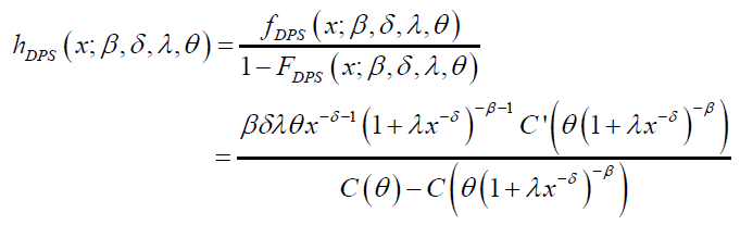
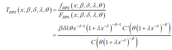
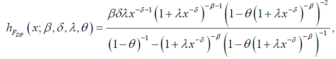
The hazard and reverse hazard functions for DP distribution are given by:
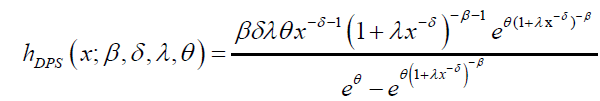
and
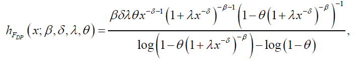
respectively. Likewise, the hazard and reverse hazard functions for DG distribution are given by:
and
respectively. The hazard and reverse hazard functions for the DL distribution are given by:
and
respectively. The hazard and reverse hazard functions for DB distribution are given by:
and
respectively.
The qth quantile of the DPS distribution is given by:
 (19)
(19)
where U ÃÆÃÂÃâââ¬Å¾ (0,1) and C-1(.) is the inverse function of C(.), Consequently, a random number can be generated based on equation (19).
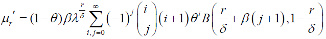
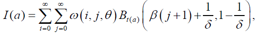
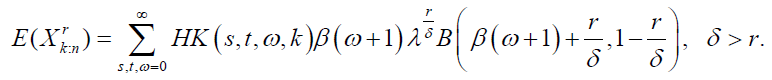
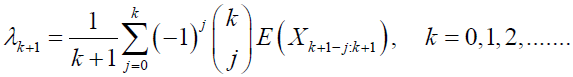
Moments are necessary and crucial in any statistical analysis, especially in applications. Moments can be used to study the most important features and characteristics of a distribution (e.g., tendency, dispersion, skewness and kurtosis). If the random variable X has a DPS distribution, with parameter vector θ=(λ, δ, β, θ); then the rth moment of X is given by:
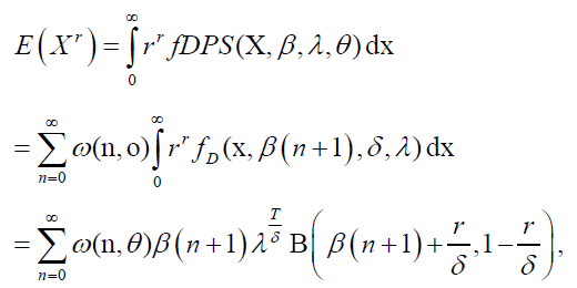 (20)
(20)
for δ>r. Note that the rth non-central moment follows readily from the fact that DPS pdf can be written as a linear combination of Dagum densities with parameters λ, β (n+1),δ>0.
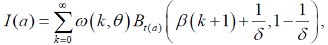
The rth conditional moment for DPS distribution is given by:
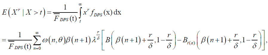 (21)
(21)
Where  The mean residual life function is
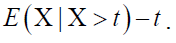
The amount of scattering in a population can be measured to some extent by the totality of deviations from the mean and the median. In this section, the mean and median deviations, as well as Bonferroni and Lorenz curves of the DPS distribution are presented. If X has the DPS distribution, we can derive the mean deviation about the mean μ=E(X) and the mean deviation about the median M from

respectively. The mean μ is obtained from equation (20) with r=1, and the median M is given by equation (19) when q=1/2. The measure δ1 and δ2 can be calculated by the following relationships:
 (22)
(22)
where 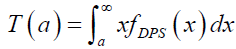 is given by:

and  then Bonferroni, B(p) and Lorenz, L(p) curves are given by:
respectively,  The mean of the DPS distribution is obtained from equation (20) with r=1 and the quantile function is given in equation (19). Consequently,
 (23)
(23)
 is incomplete Beta function.
In this section, the distribution of the kth order statistic and Renyi entropy for the DPS distribution are presented. The entropy of a random variable is a measure of variation of the uncertainty.
Order Statistics
The pdf of the kth order statistics from a pdf f(x) is
 (24)
(24)
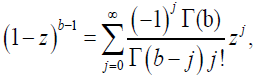
We apply the series expansion
 (25)
(25)
for b>0 and |z<1, to obtain the series expansion of the distribution of order statistics from DPS distribution. Using equations (25), the pdf of the kth order statistic from DPS distribution is given by:
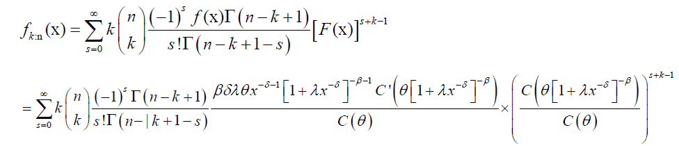 (26)
(26)
Renyi entropy of a distribution with pdf f(x) is defined as:
Note that by using equation (6), we have:
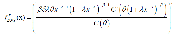 (27)
(27)
Consequently, Renyi entropy of DPS distribution is given by:
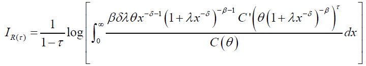
Renyi entropy for the special cases can be readily obtained for specified C(θ).
In this section, we discuss several methods of estimation of the model parameters including maximum likelihood, ordinary least squares, weighted least squares, minimum distance and maximum product of spacing. The method of maximum likelihood is presented in detail.
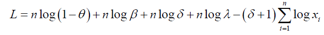
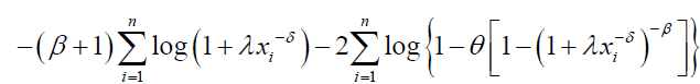
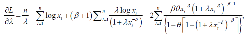
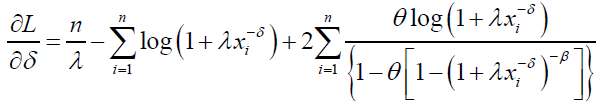
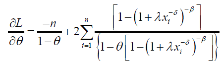
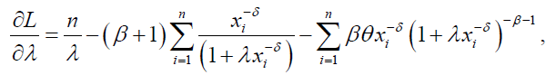
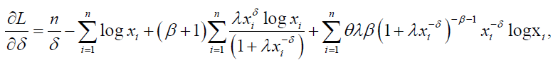
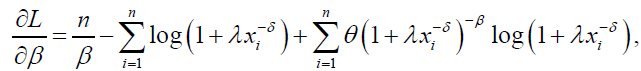
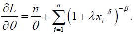
Estimation of the unknown parameters of the DPS distribution by the method of maximum likelihood is addressed in this section. Let x1,…, xn be a random sample of size n from DPS distribution and θ=(β,δ,λ,θ)T be the parameter vector. The loglikelihood function for _ based on this sample becomes
 (28)
(28)
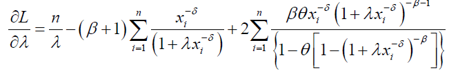
The score components corresponding to the parameters in θ are given by:
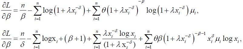
And,
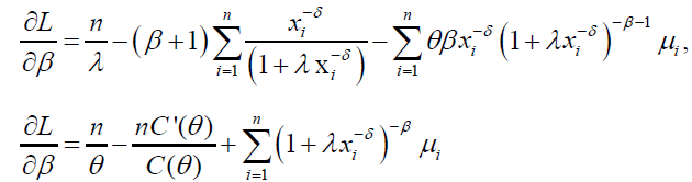 (29)
(29)
where 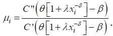 The Maximum Likelihood Estimator (MLE),
 can be obtained by solving simultaneously the nonlinear equations”.
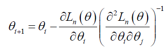
These are not linear in the parameters. Hence iterative methods are required to solve them. The Newton-Raphson method is an iterative method for solving nonlinear equations. To implement the Newton-Raphson method we require the second partial derivatives of log-likelihood function (28). The second partial derivatives are obtained as
 (30)
(30)
Note that (30) is a matrix called the Hessian matrix. In the Newton-Raphson method, provisional estimates for the vector of parameters θ on iteration ‘i’ are improved by:
These iterations continue until the changes in the parameter estimates and/or likelihood value are sufficiently small. At this point, the solution is said to have converged, and the large-sample variance-covariance matrix of the maximum likelihood estimator is then obtained as the negative inverse of the matrix of second derivatives. Standard errors of the parameter estimates are obtained as the square root values of the diagonal entries of this (negative inverse) matrix. The maximum likelihood estimates and their accompanying standard errors can be used to compute asymptotic z-statistics (i.e., Wald statistics) or construct confidence intervals.
In this subsection, we discuss the method of both ordinary least squares and Weighted Least Squares. Let x1:n<x2:n<…<xn:n denote the order statistics based on a random sample of size n from the distribution with CDF F(y), then
 (31)
(31)
Now, let  denote the order statistics based on a random sample of size n from the DPS distribution. The Ordinary Least Square (OLS) estimates of the DPS parameters
 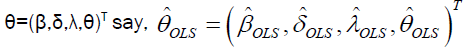 are obtained by minimizing the function
 (32)
(32)
The Weighted Least Square (WLS) estimates of the DPS parameters  are obtained by minimizing the function
 (33)
(33)
where 
The estimates of the DPS parameters can be obtained via the minimization of the well-known Anderson-Darling and Cramervon Mises goodness-of-_t statistics. This class of goodness-of-_t statistics is based on the difference between the estimates of the DPS CDF and the corresponding empirical distribution function. The Anderson-Darling (AD) estimates of the DPS model parameters θAD, say are obtained by minimizing the function
 (34)
(34)
The Cramer-von Mises (CVM) estimates of the DPS parameters  are obtained by minimizing the function
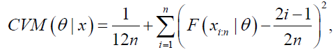 (35)
(35)
with respect to the parameters θ=(β, δ, λ, θ)T.
The (n+1) uniform spacings of the first order of the sample are given by D1=F(x1:n|θ), Dn+1=1-F(xn:n|θ) and Di=F(xi:n| θ)- F(x(i-1):n| θ); i=1,2,…, n: The Maximum Product of Spacings (MPS) method consist of finding the values of θ which maximizes the geometric mean of the spacings given by:
 (36)
(36)
or equivalently,
 (37)
(37)
by taking  The MPS estimates of the parameters, denoted by
 is obtained by solving the nonlinear equations
using a numerical method. See Chen and Amin [20] for additional details.
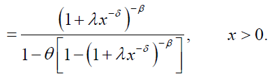
In this section, we consider and study Dagum-geometric and Dagum-Poisson distributions in detail. We focus on the case in which N is a discrete random variable following a geometric distribution (truncated at zero) with the probability mass function given by
 (38)
(38)
Note that N can also be taken to follow other discrete distributions, such as binomial, Poisson, logarithmic, where the discrete distribution need to be truncated zero because one must have N ≥ 1. Now, let X1,X2,….,XN be N independent and identically distributed (iid) random variables following the Dagum distribution cumulative distribution function. If then the conditional cumulative distribution of X(1)|N=n is given by:
and the CDF of X(1) is given by:
 (39)
(39)
Note that with  then the conditional cumulative distribution of X(N)|N=n is given by:
and the CDF of X(N) is given by:
 (40)
(40)
The corresponding pdf of X(1) is given by:
 (41)
(41)
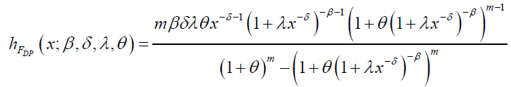
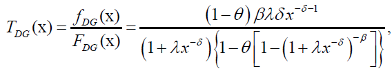
We shall refer to the distribution given by equations (40) and (41) as the Dagum geometric (DG) CDF and pdf, respectively. The Hazard Function (HF) and Reverse Hazard Functions (RHF) of the DG distribution are given by:
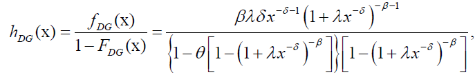 (42)
(42)
and
 (43)
(43)
respectively. The plots of DG pdf and hazard rate function for selected values of the model parameters λ, δ, β and θ are given in Figures 1 and 2.

Figure 1. Graphs of DG pdf.

Figure 2. Graphs of DG hazard functions.
These plots of the hazard function show various shapes including monotonically decreasing, unimodal and upside down bathtub shapes for different combinations of the values of the parameters. The density and hazard functions can exhibit different behavior depending on the values of the parameters when chosen to be positive, as shown in these plots (Figures 1 and 2). However, it is hard to analyze the shape of both the density and hazard function due to their complicated forms. The plots of the hazard rate function show various shapes including monotonic and non-monotonic shapes such as upside down bathtub shapes for the combinations of the values of the parameters. This flexibility makes the DG hazard rate function suitable for both monotonic and non-monotonic empirical hazard behaviors that are likely to be encountered in real life situations.
Let N be distributed according to the zero-truncated Poisson distribution
with PDF
 (44)
(44)
Let X=max(Y1,….,YN), then the CDF of X|N=n is given by:
 (45)
(45)
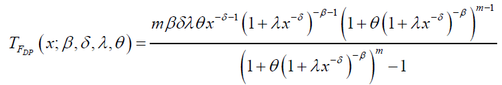
which is the Dagum distribution with parameters λ, δ, and nβ: The Dagum-Poisson (DP) distribution denoted by DP (λ, δ, β, θ) is defined by the marginal CDF of X, that is,
 (46)
(46)
for x>0, λ, β, δ, θ>0. The DP density function is given by:
 (47)
(47)
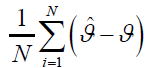
The plots of DP pdf and hazard rate function for selected values of the model parameters λ, δ, β and θ are given in Figures 3 and 4.

Figure 3. Graphs of DP PDF.

Figure 4. Graphs of DP hazard functions.
The plots of the hazard function show various shapes including monotonically decreasing, unimodal and bathtub followed by upside-down bathtub, upside down bathtub shapes for different combinations of the values of the parameters.
The DG distribution is a very flexible model that has several different sub-models when its parameters are changed. The DG distribution contains several sub-models including the following distributions.
• If β=1, then DG distribution reduces to a new distribution called Log-Logistic Geometric (LLoGG) or Fisk Geometric (FG) distribution with CDF given by:
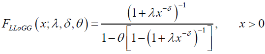 (48)
(48)
If in addition to β=1; we have θ↓0, then the resulting distribution is the log-logistic or Fisk distribution.
• When θ↓0 in the DG distribution, we obtain Dagum distribution
• The Burr-III geometric (BIIIG) distribution is obtained when λ=1: If in addition, θ↓0, the Burr-III distribution with parameter δ,β>0 is obtained
The DP distribution contains several special-models including the following distributions.
• If β=1; then DP distribution reduces to a new distribution called Log-Logistic Poisson (LLoGP) or Fisk-Poisson (FP) distribution with CDF given by:
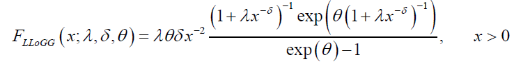 (49)
(49)
If in addition to β=1; we have θ↓0, then the resulting distribution is the log-logistic or Fisk distribution.
• When θ↓0 in the DP distribution, we obtain Dagum distribution
• The Burr-III Poisson (BIIIP) distribution is obtained when λ=1: If in addition, θ↓0, Burr-III distribution with parameter δ,β>0 is obtained
In this subsection, some statistical properties of DG and DP distributions including quantile function, moments, conditional moments, Lorenz and Bonferroni curves are presented.
In this subsection, we provide an expansion of the DG distribution. Note that, using the fact that if |z<1 and k>0, we have the series representation
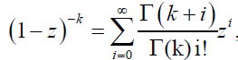 (50)
(50)
and the binomial expansion [1-(1+λx-δ)-β]i given by:
 (51)
(51)
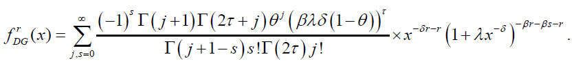
the DG pdf can be written as follows:
 (52)
(52)
where  is the Dagum pdf with parameters
λ, β (j+1),δ>0. The above equation shows that the DG density is indeed a linear combination of Dagum densities. Consequently, the mathematical and statistical properties can be immediately obtained from those of the Dagum distribution.
Similarly, applying the fact that Maclaurin series expansion of  the DP pdf can be written as follows:
 (53)
(53)
where  is the Dagum pdf with parameters λ, β (k+1), δ>0. The above equation shows that the DP density is indeed a linear combination of Dagum densities.
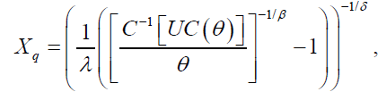
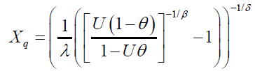
The qth quantile of the DG distribution is obtained by solving the nonlinear equation  , where U is a uniform variate on the unit interval [21]. It follows that the qth quantile of the DG distribution is given by
Similarly, the qth quantile of the DP distribution is obtained by solving the nonlinear equation 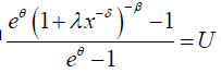 where U is a uniform variate on the unit interval [21]. It follows that the qth quantile of the DP distribution is given by:
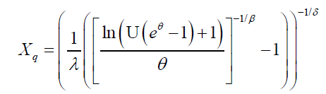 (55)
(55)
Consequently, the random number can be generated based on equation (55).
In this subsection, we present the rth moment of DG and DP distributions. The rth moment of the DG distribution is given by:
 (56).
(56).
The Moment Generating Function (MGF) of X is given by:

Similarly, the rth moment of the DP distribution is given by:
 (57)
(57)
For income and lifetime distributions, it is of interest to obtain conditional moments and mean residual life function. The rth conditional moments for DG distribution is given by:

where  The mean residual life function is E (X|X>t)-t.
Similarly, the conditional moments for DP distribution is given by:
 (58)
(58)
where  The mean residual life function is E (XjX>t) –t.
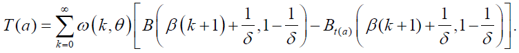
If X has the DG distribution, we can derive the mean deviation about the mean μ=E(X) and the mean deviation about the median M from equation 22, that is,

where the mean μ is obtained from equation (56) with r=1, the median M is given by equation (54) when q=1/2 , and

Also, the measure δ1 and δ2 for the DP distribution can be calculated by the following relationships:
 (59)
(59)
where  follows from equation (58), that is,
Bonferroni and Lorenz curves are a widely used tool for analyzing and visualizing income inequality. Lorenz curve, L(p) can be regarded as the proportion of total income volume accumulated by those units with income lower than
or equal to the volume p, and Bonferroni curve, B(p) is the scaled conditional mean curve, that is, the ratio of group mean income of the population. Let and μ=E(X), then Bonferroni and Lorenz curves are given by
  and
and respectively, for 0 ≤ p ≤ 1, and
  The mean of the DG distribution is obtained from equation (56) with r=1 and the quantile function is given in equation (54). Consequently,
for δ>1, where is incomplete Beta function.
Similarly, for the DP distribution, we have:
for δ>1, where  is incomplete Beta function.
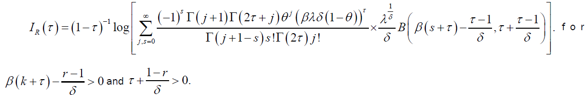
In this section, the distribution of the kth order statistic, L-moments [22] and Renyi entropy for the DG and DP distributions are presented. The entropy of a random variable is a measure of variation of the uncertainty.
We apply the series expansion
 (62)
(62)
For b>0 and |z|<1, and equation (50), to obtain the series expansion of the distribution of order statistics from DG distribution. The pdf of the kth order statistic from DG distribution (using equation (26)) is given by:
where 
The rth moment of the distribution of the kth order statistics from the DG distribution is given by:
 (63)
(63)
For δ>r; where  is the complete beta function.
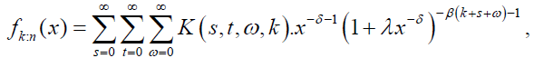
Similarly, the pdf of the kth order statistic from DP distribution is given by:

That is,
where  Thus, the pdf of the ith order statistic from the DP distribution is a linear combination of Dagum pdfs with parameters λ, β (w+1) and δ>0. The rth moment of the distribution of the ith order statistic is given by:
The L-moments [22] are expectations of some linear combinations of order statistics and they exist whenever the mean of the distribution exits, even when some higher moments may not exist. They are relatively robust to the effects of outliers and are given by:
 (65)
(65)
The L-moments of the DG and DP distributions can be readily obtained from equation (65). The first four L-moments are given by respectively.
Note that by using equation (62), we have,
 (66)
(66)
Renyi entropy of DG distribution is given by:
In this section, we consider the Maximum Likelihood Estimators (MLE's) of the parameters of the DG and DP distributions. Let x1,…, xn be a random sample of size n from DG or DP distribution and Θ=(λ, δ, β, θ)T be the parameter vector. The log-likelihood function for the DG distribution can be written as:
 (67)
(67)
The associated score function is given by 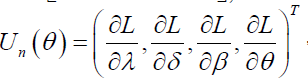 where
where
 (69)
(69)
 (70)
(70)
and
 (71)
(71)
The Maximum Likelihood Estimate (MLE) of Θ, say  , is obtained by solving the nonlinear system Un(Θ)=0. The solution of this nonlinear system of equation is not in a closed form. These equations cannot be solved analytically, and statistical software can be used to solve them numerically via iterative methods. We can use iterative techniques such as a Newton-Raphson type algorithm to obtain the estimate
The log-likelihood function for the DP distribution can be written as:
 (72)
(72)
The associated score function is given by:
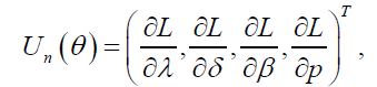
where
 (73)
(73)
 (74)
(74)
 (75)
(75)
and
 (76)
(76)
The Maximum Likelihood Estimate (MLE) of Θ, say , is obtained by solving the nonlinear system Un(θ)=0: The solution of this nonlinear system of equation is not in a closed form. These equations cannot be solved analytically, and statistical software can be used to solve them numerically via iterative methods. We can use iterative techniques such as a Newton-Raphson type algorithm to obtain the estimate of Θ.
In this section, we present the asymptotic confidence intervals for the parameters of the DG and DP distributions. The expectations in the Fisher Information Matrix (FIM) can be obtained numerically. Let 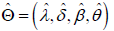 be the maximum likelihood estimate of Θ = (λ,α ,β ,θ ) . Under the usual regularity conditions and that the parameters are in the interior of the parameter space, but not on the boundary, we have
 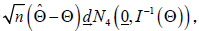 where I(Θ) is the expected Fisher information matrix. The asymptotic behavior is still valid if I(Θ) is replaced by the observed information matrix evaluated at that is
 . The multivariate normal distribution with mean vector
0=(0, 0, 0, 0)T and covariance matrix I-1(Θ) can be used to construct confidence intervals for the model parameters. That is, the approximate 100 (1-η)% two-sided confidence intervals for λ, δ, β and θ are given by:
 respectively, where
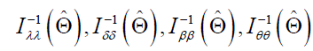 are diagonal elements of
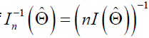 and Zη/2 is the upper (η/2)th percentile of a standard normal distribution.
We can use the Likelihood Ratio (LR) test to compare the fit of the DG or DP distribution with its sub-models for a given data set. For example, to test θ=0; the LR statistic is 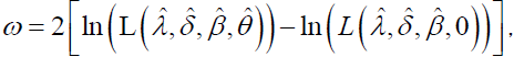 where
where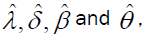 are the unrestricted estimates, and
 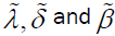 are the restricted estimates. The LR test rejects the null hypothesis if
 where
where denote the upper 100ÃÆÃÂÃâââ¬Å¾% point of the χ2 distribution with 1 degrees of freedom.
In this section, a simulation study is conducted to assess the performance and examine the mean estimate, average bias, root mean square error of the maximum likelihood estimators and width of the confidence interval for each parameter. We study the performance of the DP distribution by conducting various simulations for different sample sizes and different parameter values. Equation (55) is used to generate random data from the DP distribution.
The simulation study is repeated for N=5,000 times each with sample size n=25, 50, 75, 100, 200, 400, 800 and parameter values I: λ=2:5, β=0:6, δ=1:5, θ=0:8 and II: λ=3:8, β=0:5, δ=0:2, θ=1:2. Five quantities are computed in this simulation study.
Mean estimate of the MLE  of the parameter ϑ = λ,δ ,β ,θ :

Average bias of the MLE of the parameter ϑ = λ,δ ,β ,θ :
 .
.
Root mean squared error (RMSE) of the MLE of the parameter ϑ = λ,δ ,β ,θ :
Coverage probability (CP) of 95% confidence intervals of the parameter ϑ = λ,δ ,β ,θ , i.e., the percentage of intervals that contain the true value of the parameter ϑ
Average width (AW) of 95% confidence intervals of the parameter ϑ = λ,δ ,β ,θ
Table 2 presents the Mean, Average Bias, RMSE, CP and AW values of the parameters λ, δ, β and θ for different sample sizes. From the results in Table 2, we can verify that as the sample size n increases, the RMSEs decay toward zero. We also observe that for all the parametric values, the biases decrease as the sample size n increases. The table shows that the coverage probabilities of the confidence intervals are reasonably close to the nominal level of 95% and the average confidence widths decrease as the sample size n increases. Consequently, the MLE's and their asymptotic results can be used for estimating and constructing confidence intervals even for reasonably small sample sizes.
| l | ll | ||||||||||
|---|---|---|---|---|---|---|---|---|---|---|---|
| Parameter | n | Mean | Average bias | RMSE | CP | AW | Mean | Average bias | RMSE | CP | AW |
| λ | 25 | 6.1059 | 3.6059 | 12.8314 | 0.9208 | 57.6441 | 10.4999 | 6.6999 | 18.0013 | 0.9442 | 99.1421 |
| 50 | 4.1516 | 1.6516 | 8.4074 | 0.881 | 29.089 | 7.3514 | 3.5514 | 12.0537 | 0.9074 | 53.1391 | |
| 75 | 3.21 | 0.7097 | 5.2219 | 0.85 | 18.9689 | 6.2794 | 2.4794 | 9.2801 | 0.8894 | 38.5516 | |
| 100 | 2.7732 | 0.2732 | 3.3678 | 0.8226 | 14.5403 | 5.425 | 1.625 | 7.2022 | 0.8694 | 29.5216 | |
| 200 | 2.3204 | -0.1796 | 1.8215 | 0.8004 | 9.7076 | 4.4593 | 0.6593 | 3.9145 | 0.875 | 18.3216 | |
| 400 | 2.233 | -0.267 | 1.2408 | 0.8102 | 7.3836 | 4.1527 | 0.3527 | 2.5355 | 0.8794 | 12.898 | |
| 800 | 2.2742 | -0.2258 | 0.9722 | 0.8288 | 5.8144 | 4.0522 | 0.2522 | 1.8465 | 0.8846 | 9.2902 | |
| β | 25 | 0.581 | -0.019 | 0.7345 | 0.8916 | 3.2394 | 0.4635 | -0.03646 | 0.5781 | 0.9178 | 2.3821 |
| 50 | 0.5124 | -0.0876 | 0.3648 | 0.8966 | 1.5152 | 0.4205 | -0.0795 | 0.3546 | 0.9174 | 1.2299 | |
| 75 | 0.5076 | -0.0924 | 0.2996 | 0.9064 | 1.2018 | 0.4151 | -0.0849 | 0.2097 | 0.9174 | 0.9724 | |
| 100 | 0.5039 | -0.0961 | 0.2318 | 0.9126 | 1.0504 | 0.4207 | -0.0793 | 0.1729 | 0.9168 | 0.8574 | |
| 200 | 0.5205 | -0.0795 | 0.1765 | 0.9326 | 0.7726 | 0.4395 | -0.0605 | 0.1421 | 0.9316 | 0.6306 | |
| 400 | 0.5447 | -0.0553 | 0.1333 | 0.9408 | 0.536 | 0.4615 | -0.0385 | 0.1131 | 0.9446 | 0.4499 | |
| 800 | 0.5673 | -0.0327 | 0.092 | 0.9532 | 0.3613 | 0.4797 | -0.0203 | 0.0779 | 0.9682 | 0.3066 | |
| δ | 25 | 1.7356 | 0.2356 | 0.5704 | 0.987 | 2.2488 | 0.2314 | 0.0314 | 0.0708 | 0.9892 | 0.3004 |
| 50 | 1.6076 | 0.1076 | 0.3801 | 0.9776 | 1.5019 | 0.2155 | 0.0155 | 0.0489 | 0.9834 | 0.2054 | |
| 75 | 1.55 | 0.05 | 0.2914 | 0.9698 | 1.2069 | 0.2097 | 0.0097 | 0.0408 | 0.9734 | 0.1672 | |
| 100 | 1.5211 | 0.0211 | 0.2487 | 0.9672 | 1.0362 | 0.2064 | 0.0065 | 0.0343 | 0.9756 | 0.1446 | |
| 200 | 1.4842 | -0.0158 | 0.1742 | 0.9466 | 0.7559 | 0.2017 | 0.0017 | 0.0242 | 0.963 | 0.1044 | |
| 400 | 1.4775 | -0.0225 | 0.1294 | 0.9424 | 0.5591 | 0.2001 | 0.0001 | 0.01797 | 0.9554 | 0.0762 | |
| 800 | 1.482 | -0.018 | 0.094 | 0.9506 | 0.4134 | 0.1997 | -0.0003 | 0.0129 | 0.9548 | 0.0553 | |
| θ | 25 | 2.0443 | 1.2443 | 1.825 | 0.9422 | 14.2042 | 2.1845 | 0.9847 | 1.6176 | 0.976 | 14.1843 |
| 50 | 2.1779 | 1.3779 | 2.005 | 0.9508 | 12.4729 | 2.2855 | 1.0855 | 1.806 | 0.9828 | 12.2621 | |
| 75 | 2.1795 | 1.3795 | 2.085 | 0.948 | 11.5404 | 2.2897 | 1.0897 | 1.9271 | 0.988 | 11.4679 | |
| 100 | 2.2186 | 1.4186 | 2.1324 | 0.957 | 10.8672 | 2.2543 | 1.0543 | 1.897 | 0.9912 | 10.5053 | |
| 200 | 2.0282 | 1.2282 | 1.9951 | 0.9748 | 9.1258 | 2.0514 | 0.8514 | 1.7881 | 0.9942 | 8.3227 | |
| 400 | 1.7006 | 0.9006 | 1.6196 | 0.9804 | 6.8676 | 1.7566 | 0.5566 | 1.469 | 0.9938 | 6.1189 | |
| 800 | 1.3582 | 0.5582 | 1.1099 | 0.9682 | 4.9404 | 1.4705 | 0.2706 | 1.0325 | 0.9854 | 4.2113 | |
Table 2. Monte carlo simulation results: mean, average bias, RMSE, CP, and AW.
In this section, we present an example to illustrate the edibility of the DG and DP distributions and its sub-models for data modeling. Estimates of the parameters of DG distribution (standard error in parentheses), Akaike Information Criterion (AIC), Bayesian Information Criterion (BIC) and Kolmogorov-Smirnov (KS) are presented for each data set. The command NLP in SAS and the R package are used here. We also compare DG distribution with other distributions including Exponentiated Weibull Geometric (EWG) distribution and Exponentiated Weibull-Poisson (EWP) (Mahmoudi and Sephadar, [23] distribution. The CDF of the EWG and EWP distributions are given by
 (77)
(77)
and
 (78)
(78)
We also fitted the four parameter sub-model of the beta Weibull geometric (BWG) distribution given by:
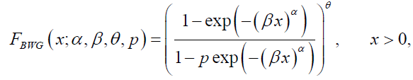 (79)
(79)
To the failure times, data set. Plots of the _tted densities and the histogram of the data are given in Figure 5. Probability plots [24] are also presented in Figure 5. For the probability plot, we plotted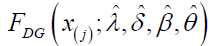 against j-0:375/n+0:25, j=1, 2, ….,n, where x(j) are the ordered values of the observed data. We also computed a measure of closeness of each plot to the diagonal line. This measure of closeness is given by the sum of squares

Figure 5. Graphs of failure times.
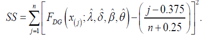 (80)
(80)
This data set represents the failure times of 50 components (per 1000h) from Murthy et al. [25], Weibull models (Vol. 505), page 180. Initial value for DG model in R code are λ=1, δ=1, β=1, θ=0.1. Estimates of the parameters of DG distribution and its related sub-models (standard error in parentheses), AIC, BIC, SS and KS for failure times data are given in Table 3. The estimated variance-covariance matrix for DG model is
| Estimates | Statistics | ||||||||
|---|---|---|---|---|---|---|---|---|---|
| Model | λ | δ | β | θ | -2logL | AIC | BIC | SS | KS |
| DG | 756914.7 | 4.9705 | 0.1363 | 0.7528 | 201.21 | 209.21 | 216.86 | 0.11 | 0.09 |
| (0.0000002) | -0.403 | -0.0319 | -0.1486 | ||||||
| FG | 6.9602 | 0.9108 | 1 | 0.8391 | 210.97 | 216.97 | 222 .71 | 0.1788 | 0.1354 |
| -0.0009 | -0.1033 | (-) | (0.041) | ||||||
| F | 1.1200 | 0.9108 | 1 | 0 | 210.97 | 214.97 | 218.79 | 0.1788 | 0.1355 |
| (0.2858) | -0.1033 | (-) | (-) | ||||||
| D | 42293.26 | 4.4033 | 0.0949 | 0 | 206.59 | 212.59 | 218.33 | 0.1867 | 0.0986 |
| (0.000002) | -0.2664 | -0.0134 | (-) | ||||||
| BIIIG | 1 | 0.8915 | 1.0598 | 0 | 211.03 | 217.03 | 222 .76 | 0.1822 | 0.1407 |
| (-) | -0.1788 | -0.4826 | (-) | ||||||
| Biil | 1 | 0.8915 | 1.0598 | 0 | 211.03 | 215.03 | 218.85 | 0.1822 | 0.1407 |
| (-) | -0.1091 | -0.1627 | (-) | ||||||
| α | β | θ | p | ||||||
| B\.YG | 0.4438 | 0.6937 | 8.9834 | 0.8926 | 203.77 | 211.77 | 219.41 | 0.2066 | 0.1557 |
| -0.1639 | -1.0563 | -31.151 | -0.3603 | ||||||
| α | β | θ | ϒ | ||||||
| EWG | 5.9525 | 28.7391 | 0.4315 | 0.2698 | 205.41 | 213.41 | 221.06 | 0.1737 | 0.1262 |
| (2.2754) | -0.1522 | (0.452) | -0.0241 | ||||||
| α | β | ϒ | θ | ||||||
| EWP | 0.0139 | 0.4972 | 0.6020 | 84.9653 | 204.91 | 212.91 | 220 .56 | 0.1580 | 0.1031 |
| -0.0267 | -1.4189 | -0.6779 | -0.0048 | ||||||
Table 3. Estimates of models for failure times data set.
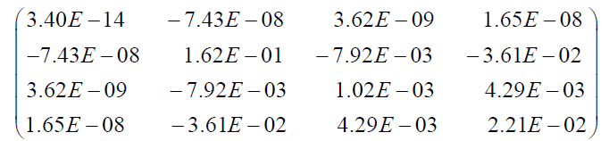
The 95% two-sided asymptotic confidence intervals for λ, δ, β and θ are given by 756914.7 ± 0.000000392, 4.9705 ± 0.7899, 0.1363 ± 0.0.0625, and 0.7528 ± 0.2913, respectively.
The LR test statistics of the hypothesis H0: FG vs Ha: DG and H0: BIIIG vs Ha: DG are 9.7594 (p-value=0.001784) and 9.8160 (p-value=0.00173). The DG distribution is significantly better than FG and BIIIG distributions. Also, the DG distribution is significantly better than D distribution based on the LR test. The values of the statistics AIC, BIC and KS when compared to those for the sub-models and non-nested EWG, EWP and BWG models also points to DG distribution as a very good _t for the failure times data. The graphs of the fitted densities, probability plots and survival suction also shows that the DG distribution is indeed the “best" model for the failure times data set.
This data set consists of 101 observations corresponding to the failure times of Kevlar 49/epoxy strands with pressure at 90% [26-31]. The failure times in hours was analyzed by [32]. Estimates of the parameters of DP distribution and its related submodels (standard error in parentheses) [33-38], AIC, BIC, W*, A*, SS and KS for failure times data are given in Table 4. We also use the LR test to compare the DP distribution and its sub-models [39-42].
| Estimates | Statistics | ||||||||||
|---|---|---|---|---|---|---|---|---|---|---|---|
| Model | λ | δ | β | θ | -2logL | AIC | AICC | BIC | W* | A* | SS |
| DP | 7.2834 | 3.3711 | 0.2015 | 0.3744 | 200.09 | 208.09 | 208.51 | 218.55 | 0.0657 | 0.4632 | 0.0699 |
| (6.7978) | (0.6884) | (0.0602) | (1.0496) | ||||||||
| FP | 0.0108 | 0.6444 | 1.0000 | 39.4781 | 261.40 | 267.40 | 267.82 | 275.24 | 1.1126 | 6.0129 | 1.0084 |
| (0.0015) | (0.0455) | (4.09E-05) | |||||||||
| BIIIP | 1.0000 | 2.1278 | 0.3085 | 1.7423 | 207.48 | 213.48 | 213.90 | 221.33 | 0.2039 | 1.1841 | 0.2319 |
| (0.2470) | (0.0920) | (0.8605) | |||||||||
| D | 9.0357 | 3.4267 | 0.2110 | 200.21 | 206.21 | 206.46 | 214.06 | 0.0742 | 0.4980 | 0.0809 | |
| (6.9969) | (0.6904) | (0.0548) | |||||||||
| F | 0.6240 | 1.2705 | 1.0000 | 225.37 | 229.37 | 229.49 | 234.60 | 0.5654 | 3.0709 | 0.3893 | |
| (0.0850) | (0.1069) | ||||||||||
| Bill | c | k | |||||||||
| 1.1737 | 1.6327 | 217.10 | 221.10 | 221.22 | 226.33 | 0.4401 | 2.3866 | 0.4741 | |||
| (0.0983) | (0.1637) | ||||||||||
| α | β | ω | θ | ||||||||
| EPLP | 0.7894 | 1.7952 | 0.9385 | 1.1684 | 204.44 | 212.44 | 212.86 | 222.90 | 0.1349 | 0.8141 | 0.1292 |
| (0.2025) | (0.6112) | (0.3829) | (1.2585) | ||||||||
| δ | β | ϒ | θ | ||||||||
| EWP | 0.8588 | 1.3030 | 0.8717 | 1.2662 | 204.62 | 212.62 | 213.03 | 223.08 | 0.1408 | 0.8415 | 0.1347 |
| (0.3679) | (0.7394) | (0.2408) | (1.2007) | ||||||||
Table 4. Estimates of models for kevlar strands failure times data.
The estimated variance-covariance matrix for the DP distribution is given by:
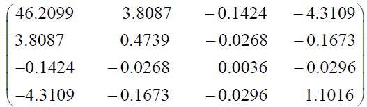
and the 95% two-sided asymptotic confidence intervals for for λ, δ, β and θ are given by 7.2834 ± 13.3269; 3.3711 ± 1.3493, 0.2015 ± 0.11799, and 0.3744 ± 2.0572, respectively.
Plots of the fitted densities and the histogram, observed probability vs predicted probability are given in Figure 6.

Figure 6. Fitted densities and probability plots for kevlar failure times.
The LR test statistics of the hypothesis H0:FP vs Ha:DP and H0:BIIIP vs Ha:DP are 61.31 (p-value<0.0001) and 7.40 (p-value=0.0065). DP distribution is significantly better than FP and BIIIP distributions. Also, the LR test indicates that DP distribution is also significantly better than Fisk and Burr-III distributions, however, there is no difference between DP and Dagum distribution based on the LR test. DP distribution has the smallest goodness of _t statistic W* and A* values as well as the smallest SS value among all the models that were fitted [43-45]. A comparison of DP distribution with the non-nested EWP and EPLP distributions using the AIC, AICC, BIC, W*, A*, and SS statistics, clearly shows that it is the superior model. Hence, DP distribution is the “best” fit for the data when compared to all the other models that were considered.
A new class of distributions called the Dagum Power Series (DPS) is proposed and studied. The DPS distribution has Dagum Poisson, Dagum geometric, Dagum logarithmic, Dagum binomial and several other distributions as special cases. The DPS distribution is exible for modeling various types of lifetime and reliability data. We also obtain closed-form expressions for the moments, conditional moments, mean deviations, Lorenz and Bonferroni curves, distribution of order statistics and Renyi entropy. Methods of finding estimators such as Minimum Distance, Maximum Product of Spacing, Least Squares, Weighted Least Squares, and Maximum Likelihood were discussed. The special cases of DG and DP distributions re-discussed in details.