Keywords |
| Diagnosis, Bond Gaph, Timed Automata, Analytic Redundancy Relations. |
INTRODUCTION |
| Supervision is a set of tools and methods used to operatea process in normal situation as well as in the presence
offailures. There is an abundance of literature on process fault diagnosis ranging from two different communities: the
SystemsDynamics and Control Engineering (FDI) community[1,2] and the Artificial Intelligence Diagnosis(DX)
community [3,4]. The two communities haveemployed different kinds of models, and made differentassumptions
concerning robustness of the generatedsolution with regard to modeling errors, measurementnoise, and disturbances.
They are quantitative model-based methods, qualitative model-based methods, and process history based-methods.The
general principle of allmodel-based FDI approaches is to compare the expectedbehavior of the system, given by model,
with its actualbehavior. The first step of a FDI procedure consists ingenerating a set of residuals. These residuals are
specialsignals that reflect the discrepancy between the twobehaviors. Analytic Redundancy Relation (ARR) methodsare
classically used for residual generation in the FDIcommunity [5]. The DX community has developedmethods such as
possible conflicts [6, 7], and analysis oftemporal causal graphs [8, 9] for diagnosis of continuoussystems. These
methods are based on the structuralanalysis of dynamic models, much like the ARR schemesdeveloped by the FDI
community. The two communitiesuse different algorithms, but the overall framework forfault isolation is similar,
defined by a two-step process: residual generation, followed byresidual evaluation[2, 3]. |
| The main purposes of this paper concern residual generationand fault isolation based on a new approach which
combined the causal graphicalapproaches (Bond graph and causal graph) and the timed automata. Thebond graph
model is used to generate systematically a setof fault indicators called also analytical redundancy relations(ARRs)deals
with the FDIaspect using Bond Graph-based modeling approach.This methodmodeling approachprovides an effective
tool for compositionalmodeling and fault detection and isolation (FDI) of dynamic systems [10], [11].ARRs are
designed; the fault detectionprocedure checks the presence of fault indicated by a non-zero value of these indicators.
We use the timed automata for locate the source of failure. In theapproach we propose here, the diagnosis system is
basedon checking the consistency between the time of failureoccurrences and the inputs sequences. It isthus necessary
to know thetime trajectories.Our method is based on the backwardexploitation of the dynamic model, where all
possiblereverse paths are searched. The reverse path is theconnection of the faulty state to the initial state. |
| This paper is organized as follows: In the next section,a proposed procedure for FDI is described. Section III andIV
give, respectively, an idea about quantitative (BG) and timed automata (TA) approaches using to developing diagnosis
approach.In Section V, An academically example is used toillustrate our approach. Finally, a conclusion is
presentedwith some perspectives. |
PROPOSED DIAGNOSIS APPROACH |
| The proposed FDI approach combines two tools: the bon graph and timed automata is shown in figure 1, where
variables u, Rarerespectively input state and the set ofresidues. |
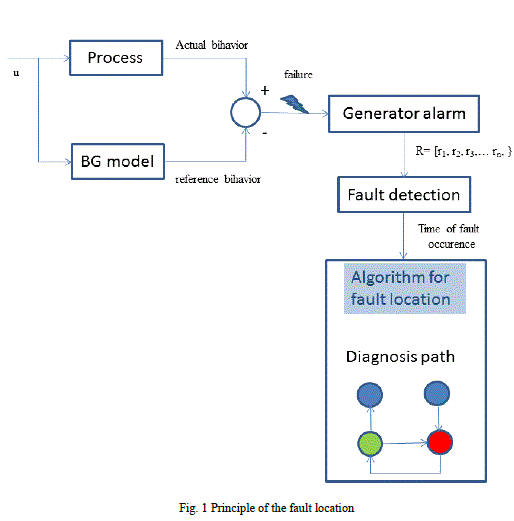 |
| The quantitative approach is based on the bond graph modelwhich allows the generation of the fault indicators and the
dynamic model (AT) which presents a tool of fault location and isolation. The diagnostic technique for fault location is
based on time analysis, where the coherent trace is searched by the verification ofelapsed time with global time of
alarm.We consider a plant equipped with an alarm andwith a global clock for synchronization. Alarmproduces an error
signal when a fault is detected. Ourdiagnosis task is to locate and identify all faults whichcan occur (figure 1). The aim
is to find the coherent diagnostic path, which corresponds to the faultyevolution of the system. |
| In our case verification (analysis) means searching accessible trace of timed automata(reverse path). This reverse path
project the evolution of the system, from a final faulty state to the initial state [12]. The reverse path is also called
diagnostic path. We suppose the initialstate is known. Our task can be seen as retrace the automaton graph from the
faulty statesto the known origin state. The aim is to find from the set of reverse path the coherent ones. |
QUANTITATIVE GRAPHICAL APPROACH |
| A. Bond graph basis |
| Bond graphs are a domain-independent graphical description of dynamic behaviour of different physicalsystems
(mechanical, electrical, hydraulic …). The basis is that bond graphs arebased on energy and energy exchange.
BGmodeling is a powerful tool for modeling engineering systems, especially when differentphysical domains are
involved. |
| The concept of bond graphs was originated by [13]. The idea was further developed byKarnopp and Rosenberg [14],
such that it could be used inpractice [15][16]. A number of methods have been developed for fault detection and
isolation. Allmethods of fault detection work by designing residual functions. The residual represents thedifference
between an estimated value and a measured one, which should be zero duringnormal operation, but large in the
presence of faults [10]. |
| 1) Generalized variables |
| Thebondgraphbased onthegraphical representation of theenergy exchangeprocesseswithin thesystem to be modelled.
These weather applicationscan then beconverted intoblock diagramormathematical formasthestate representation. This
modelling approach uses thegeneralizedvariable powerand energy as well asgeneralizedelements: resistor ( R ),
compliance ( C ), inertia ( I ), transformer (TF), gyrator (GY), effort source (Se) and flow source (Sf)the
intuitiveanalogy voltage- effort. Depending on the physical environment, these variables have different value.
Forexample in electrical networks, flow represents the “current” and effort the “voltage”, inmechanical linkages, flow
represents the “velocity” and effort the “force”. |
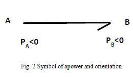
| On each Bond, one of the variables must be the cause and the other the effect. This can bededuced by the relationship
indicated by the arrow direction. Thislinkindicatesthevariablespowerandby conventionthedirection of the half arrowis
thedirectioncorresponding to the positivepoweras shown inFigure2. Effort and flow causalitiesalways act in opposite
directions in a Bond. |
 |
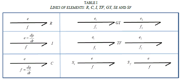
| The representations of generalized elements, R, C, I, TF, GY, Se and Sf, are shown in Table 1. The elements R, C, I are
passive, they receive energy from which the direction of their bond. TF, GY are conservative elements, they only
transfer energy where the orientation of links (incoming and outgoing).TF, GY is active elements, it provides energy,
and their bond is coming. |
 |
| 1) Junction elements |
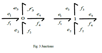
| There are only two kinds of junctions, the 1 and the 0 junction (fig. 3). They conserve power and are reversible. They
simply represent system topology and hence the underlying layer of junctions and two-port elements in a complete
model (also termed the Junction Structure) is power conserving. 0 junctions have equality of efforts while the flows
sum up to zero, if power orientations are taken positive toward the junction. 1junctions have equality of flows and the
efforts sum up to zero with the same power orientation. |
 |
| B. Generation of fault indicators |
| The diagnosis using bond graph models requires the generation of Analytical Redundancy Relations whichrepresentthe
set of constraints deduced from the model of the system containing the different known variables(measurements,
sources and parameters) [17][18]. ARR are obtained from the behavior model of the system through
differentprocedures of elimination of unknown variables.The online evaluation and analysis of these indicators allow to
detect and to isolate faults affecting the process.Numeric evaluation of each ARR is called a residual, which is used in
model basedFault Detection and Isolation (FDI) algorithms. |
| The numerical evaluation of an analytical redundancy relation led to a residual of this form: |
| r = f (K) = f (De,Df ,Se,Sf ,MSe,Sf ,u,θ ) = 0 |
| whereK is the set of known variables and/or parameters. In a bond graph sense,the set of known variables represents the
outer vertices (the flow Dfand the effortDe detectors, the flow Sfand the effort Se sources, the modulated flow
MSfandeffort MSesources, the process inputs u and the process parameters θ) [21]. |
| A residual is sensitive to faults of the jthcomponent if and only if one (or more)parameter belonging to the jthcomponent
appears inri . |
| A fault indicator algorithm is given as follows: |
| 1) Preferred derivative causality is assigned to storage elements and detectors that becomes dualized; |
| 2) Deduce equations of behavior FB, junctions FJ, measurement Fy, controlled sources FAand of controller system FC; |
| 3) Unknown variables are directly eliminated from the BG model using covering causal path rules; |
| 4) For any detector whose causality is reversed, an ARR is deduced. |
| C. Fault signature matrix |
| Once the ARRs are designed, they lead to the formulation of a binary fault signature matrix ji S which informs us on
the sensitivity of residual to the components failures of the physical process (sensors, actuators, etc) [17] [18]. The
matrixis defined as: |
 |
| The matrix S ji is called fault signature matrix which provides information on the localization and detection of a failure
during the system operation. A failure of a component is detectable if the variable associated with the component is
presented in at least an ARR, this failure is isolable if its signature is single (unique) i.e. different from the signatures of
the other components. |
| D. Fault Detection Bond Graph model |
| The main steps of the FDI bond graph based method to generate the ARRs, the residuals and the corresponding fault
signature matrix are summarized hereafter. Interested readers can find more details about the method in [23, 22]. |
| • Build the bond graph model in preferred integral causality. |
| • Put the bond graph model in preferred derivative causality (with sensor causality inversion if necessary). |
| • Write for each junction its corresponding equations. |
| • Write the constitutive equation for each bond graph element. |
| • Eliminate the unknown variables from each junction equation involving a detector (or a sensor) by covering the causal paths on the bond graph model in derivative causality. |
| • Generate the ARR, the residuals and the corresponding fault signature matrix. |
THE TIMED AUTOMATA |
| The timed automata tool [19] [20] is defined as a finite state machine with a set of continuous variables that are named
clock. These variables evolve continuously in each location of the automata, according to an associated evolution
function. As long as the system is in one state Li, the clock xi is continuously incremented. Its evolution is described by
X=1. The clocks are synchronized and change with the same step. |
| An invariant is associated to each state. It corresponds to the conditions needed to remain in the state. The number of
clocks depends on the parallelism in the system. The automata can stay in one state as long as the invariant condition is
checked. Each transition of an automata is conditioned by an event or temporization called “guard” and its execution
determines the discrete evolution of the variables according to its associated assignment. |
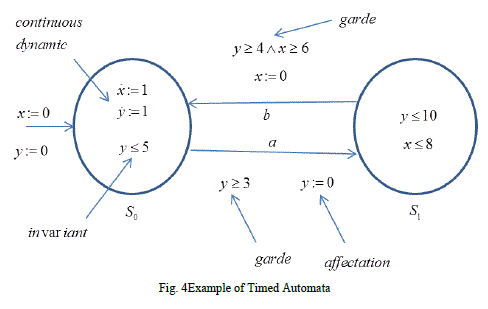
| Let us consider the timed automata given in figure 4. This automata has two clocks x and y. The continuous evolution
of time in this model is represented by x=1 and the labelled arcs in the graph represent the model of discrete
evolution. The guard in each arc is a transition labelling function that assigns firing conditions with the transitions of the automata. The affectation is a function that associates with each transition of the automata one relation that allows
actualizing the value of continuous state space variables after the firing of a transition. The invariant in the state S0 and
S1 are respectively y ≤ 5 and x ≤ 8. The initial state of this system is represented by an input arc in the origin state (S0).
In the dynamic model, active clocks are found in each state. A graphical interpretation of the timed automata is the
automata graph (Fig. 4). |
 |
| In our case verification (analysis) means searching accessible trace of timed automata(reverse path). This reverse path
project the evolution of the system, from a final faulty stateto the initial state. The reverse path is also called diagnostic
path. We suppose the initialstate is known. Our task can be seen as retrace the automaton graph from the faulty statesto
the known origin state. The aim is to find from the set of reverse path the coherent ones.
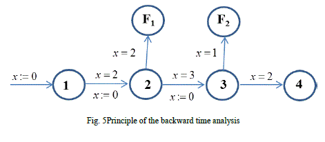
The principle of the analysis is shown in automaton graph with faultmodel (Fig.5). From fault model one can see that
fault F1 can occurs from states 2,and the fault F2 from the state 3. The diagnostic model must be defined that if fault
occursin the system, fault must be located according the time instant. If the fault occurs in thetime 4tu, it’s fault located
as F1. In another case, the fault occurs in the time 7tu, the faultF2 is located. |
 |
APPLICATION EXEMPLE |
| A. General description of the system |
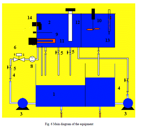
| This unit (Fig 6) consists on a hydraulic circuit, with an bottom tank (1) and asuperior process tank (2), both dual ones,
two pumps of centrifugal circulation (3),two flowmeters with a manual control valve (4), three on/off solenoid valves
(5) anda motorized proportional valve (infinitely variable) (6). Of course, together with thetubes, the union elbows,
connections, feedthroungh, main valve and the appropriatedrainage for the circuit operation. |
| As additional fixed elements, there is also a turbine flow sensor that isinstalled in one of the upward lines of flow (8),
and a temperature sensor located in alateral bottom of the process tank (9) together with a serpentine with electric
heating(11). |
| The interchangeable additional elements are an agitator (10), theimmersion level sensor should be located in the
process tank (12) and the pH sensor(solenoid), can be in the process tank or also in the second tank (13), to study
theeffect of the time out. |
 |
| B. Operation of the subsystems |
| For the level, flow and temperature control test, the liquid (water) isimpelled from the tank by the pump, located to
the left of the front of the equipment,going through the flowmeter, the solenoid valve (usually open), the motorized
valve,the turbine (flow sensor) and the process tank. It is possible to use the second pumpin the level tests, as it will be
indicated. |
| The pH control test of requires a second parallel line of flow (right),provided only with pump and a flowmeter. The
compartments of the inferior tankshould be loaded with diluted solutions of an acid and a base, respectively.
The process tank is divided in two halves, with an orifice between themthat allows their communication or isolation.
The right compartment has an overflow of variable level (that it preventsthe complete overflow of the tank, and it
allows to modify its effective liquidvolume), two drains with solenoid valves with different Cv (normally closed), and
athird one with a normal drainage valve.The left compartment is only connected to a drainage valve.
The level control tests require all the elements of the circuit and of thetank, besides the sensor located in it. In some
experiments, it is required the secondpump placed to the right-hand side of the equipment. |
| The Temperature controltests, in these cases, as we will see lateron, can be carried out with experiments in closed
circuit or in open circuit. In theclose circuit case, fill the superior tank with the right pump 1 (AB-1) and carry outthe
experiment. In open circuit, keeps a constant water flow using the pump 1, thisway, a small water flow is adjusted and the superior overflow is used as a drainagesystem. In this case, it is necessary to use the agitator to guarantee
goodtemperature uniformity. |
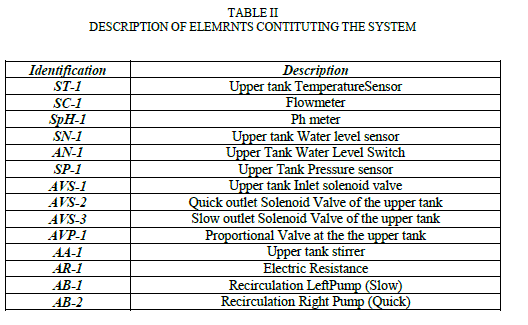
| We include in the following table II the elementsconstituting the equipment and a brief description ofeach. |
 |
| E. Fault detection based on bond graph |
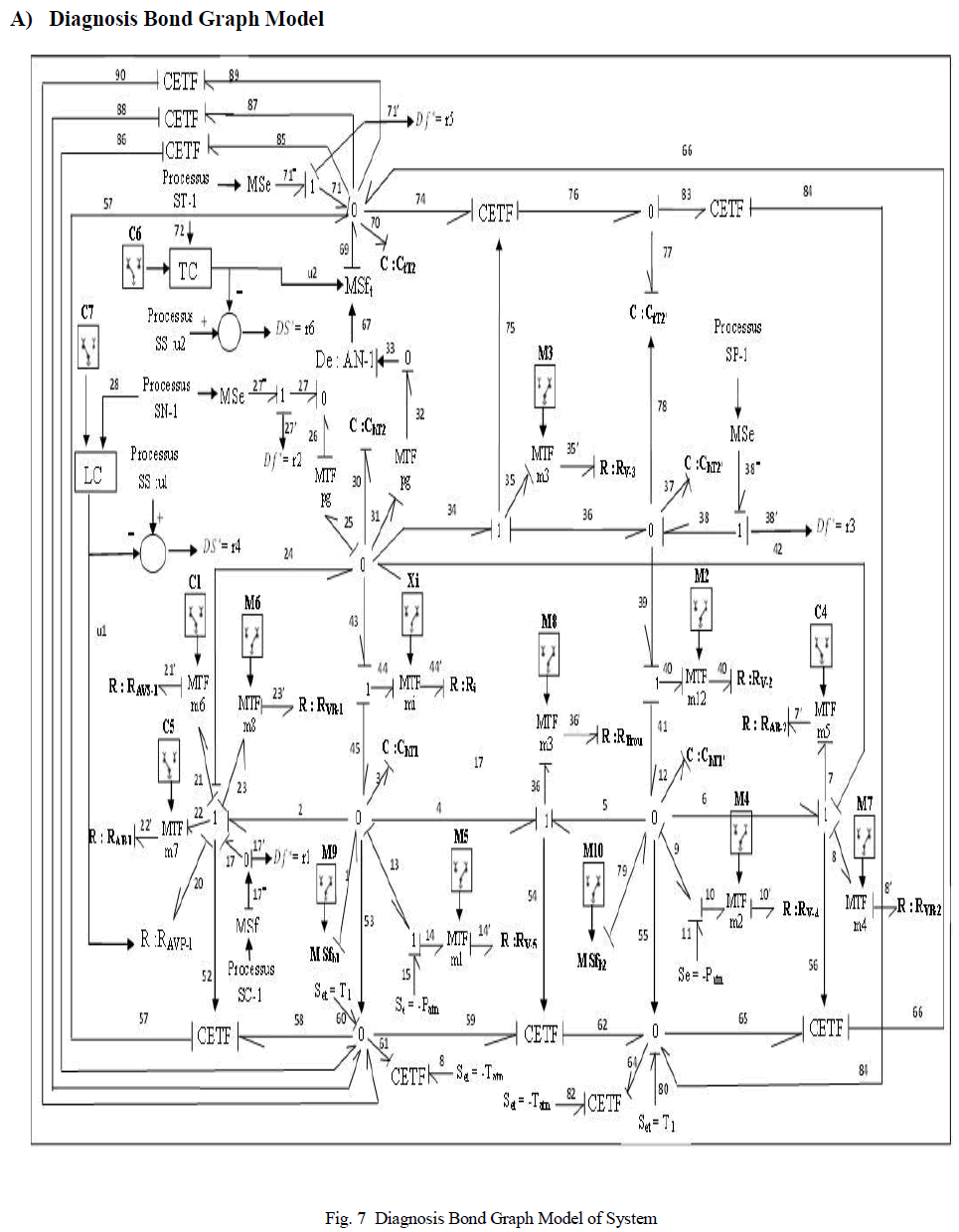
| We applied themain steps of the Fault Detection and Isolation bond graph (see §III). The bond graph model diagnosis
of the system obtained is given in figure 7 (see Appendix).It has fiveaccess points (corresponding to the five sensorsof
the system)and fiveoutputs (corresponding to the five digitalresiduesgenerated) as shown in theblockdiagram in
Figure8 |
 |
| 1) ARRs generation |
| Methods to derive ARRs from bond graph models by applyingthe causality inversion algorithm have been presentedin
[25] [16], which use structural and causal properties.The ARRs are deduced from junctions 1 and 0 that
containdetectors on the bond graph model in preferred derivativecausality, Figure 9. The unknown variables are
eliminated bycovering causal paths from detectors to unknown variables.This leads in fact to oriented graph. |
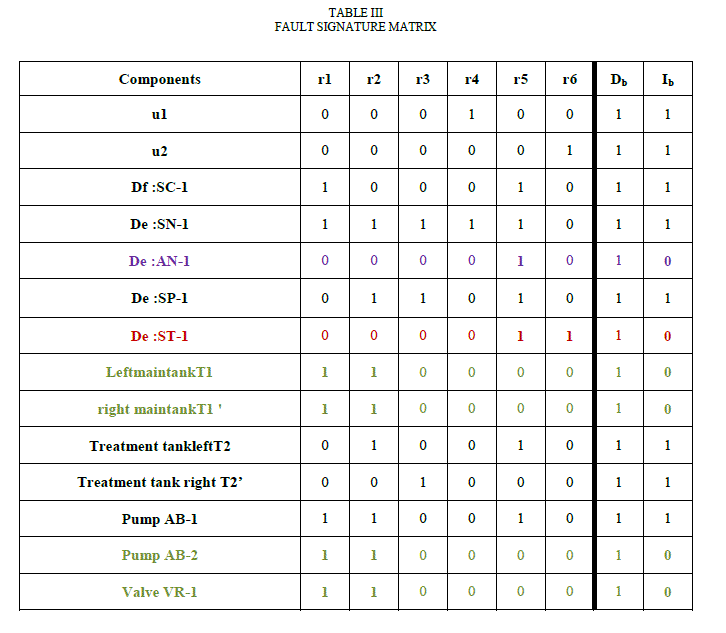
| In our case the diagnosismodelBGprovidesnumerical valuesbut alsotheresiduessignature matrixSijfailures. Indeed,itis
essentialfor the localization offailuresthat may occur duringsystem operation.The path of thecausalpathsofthe unknown
variableto the detectoris used to constructthesignature matrixfailures (Table III). Thus, aresidualriis sensitive toa failure in thecomponent jif and only ifthe variable associated withthe latteris present in thecausalpath forthe generation
ofresiduallaughed. |
| For example,thecomponents involved inthedetectorresidue r1are determined bythe followingcausalpaths: |
 |
| The components involvedin theresidue r1aregivenby the vectorK1 =[SC-1, RVR-1-1 RAVSRVR-2, RAB-1, RAB-2,
SN-1, SC-1 RAVP, tankT1, tank T1'].Thusthe application of thisprocedure on alldigitaldetectorsresiduesled to
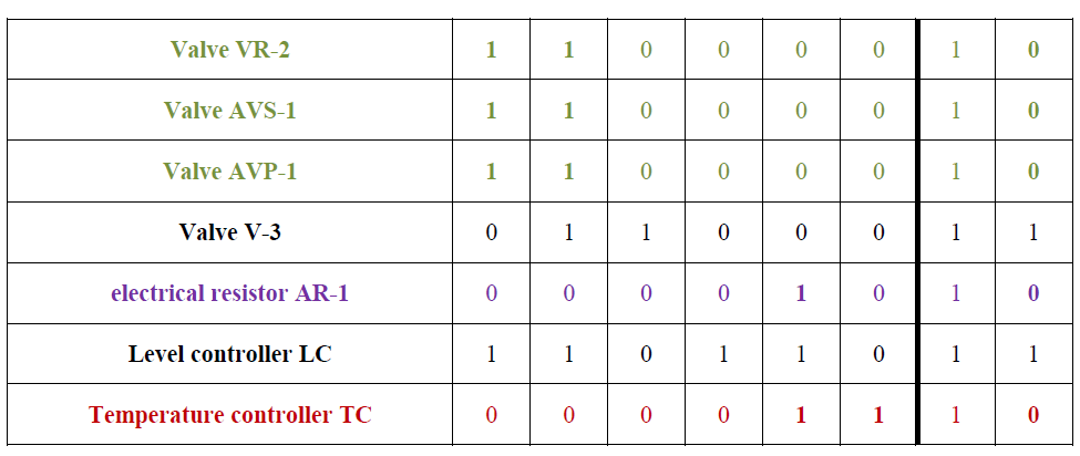
thefailuresignature matrixSij.Thefault signature matrix of the diagnosis modelis givenin TableIII |
 |
 |
| It is importantto note that thesignature matrixfaultsconstructed fromcausalpathscorresponds toa
definiteconfiguration(ormode)and thereforethe associatedmodel.Theform of the equationsfor eachelementbondgraphis
then the sameduring the whole periodof operation ina given configuration.For example, thetotal blockageof the
valveAVS-1 representedby the elementRAVS-1 causes the rupture ofallcausalpaths(andtoward) the item.
By analysing this matrix,we see thatthe variable associated witheach component ispresent in atleast one residue. So
allsystem failuresare theoreticallydetectable(= 1). |
| In addition, the signatures of componentsSN-1, SC-1, U1, U2, SP-1, AB-1, V-3, tankT2, tank T2 'and LCare
uniquemeaning thatthefailureof these componentsareisolatable(Ib = 1).
Forcons, the signatures of theST-1andTCcomponentsare identicalwhich meansthat defectsaffecting thesecomponents
cannotbe isolated(Ib= 0). |
| Our contributionin thispaperis the use oftimed automatafor the isolation ofthese non-isolablecomponentsbyBond
Graphmodel. |
| F. Fault isolation based on timed automata |
| For thephase oflocalization offaultswe consider onlypart ofthe model shown in Figure9.The goal isthe study ofthe
levelin a tankby the actionofthe valveAVP1andalsoby twosensors SN1 and AN1, respectively,measuringhighlevels
andlow. |
| We use thetimedautomatonmodeltoisolate faults insensorswhicharenotidentifiable(see TableIII). |
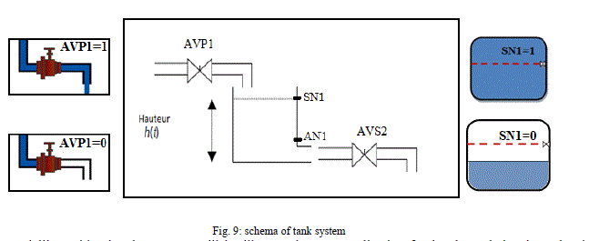 |
| Example: modelling with Timed automata will be illustrated on an application for level regulation in tank wich is
equipped by two level sensors and two valves. Valve AVP1as input valve, output valve AVS2.Figure 9, shows the
placement of two levels sensors. |
| Control: Firstly,the valve AVP1 is open; the liquidflows into tank 1.When the tank level AN1 is reached, the valve
AVS2 is is opened. Then, When the tank level SN1, the valve AVP1 is closed.. |
| Control sequence: |
| (1) S0: When the process is initialized, tank shouldbe empty. |
| (2) S1: First, valve V1 is open, a liquid flows into tank. |
| (3) S2: If level AN1 is reached then valve AVS2 is opened. |
| (4) S3: If Level SN1 is reached then AVP1 is closed. |
| The aim of backward time analysis of timed automata isto locate (isolate) a fault. In our case exploitation
meanssearching accessible trace according the time from a finalfaulty state to the initial state of automaton denoted
byreverse path. Therefore the initial state must be known.Our task can be seen as retrace the automaton graph fromthe
faulty states to the known origin state. The aim is tofind from the set of reverse path the coherent ones.
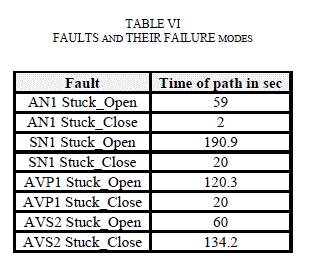
In our case whichwe considereight faultsas well as their failure modes aresummarized in Table IV. |
 |
| For these eight faultslisted, it uses onlyfivestatesdetection(S0, S1, ...,S4).Thetable V belowshowsthe conditions
necessaryto locationfault. |
 |
 |
| This algorithmbased on thetime of occurrenceof the alarm,to localizethe fault. |
| Step 1: Calculate theduration of a cycleof operation is (in our case it is 418.9sec). |
| Step2: first calculate the numberof cycles performedby the processbefore the activationof the alarm.
Number of cycles= round(talarm/418.9) |
| Step 3: Thenthe weight of thepathis calculated: Talarm-path =(418.9 *(number of cycle)) |
| Step4:comparethe value obtained withtheweight ofdifferent ways |
| In the tablebeloware listedthe weights ofdifferent paths. |
 |
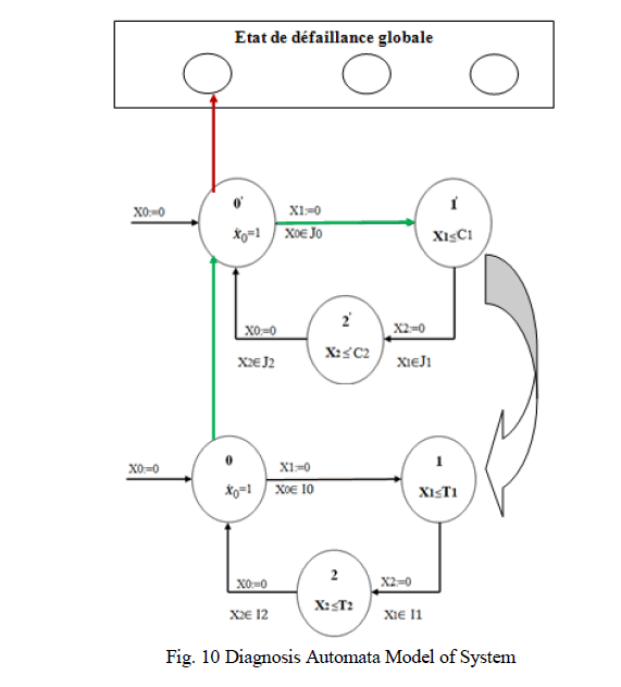
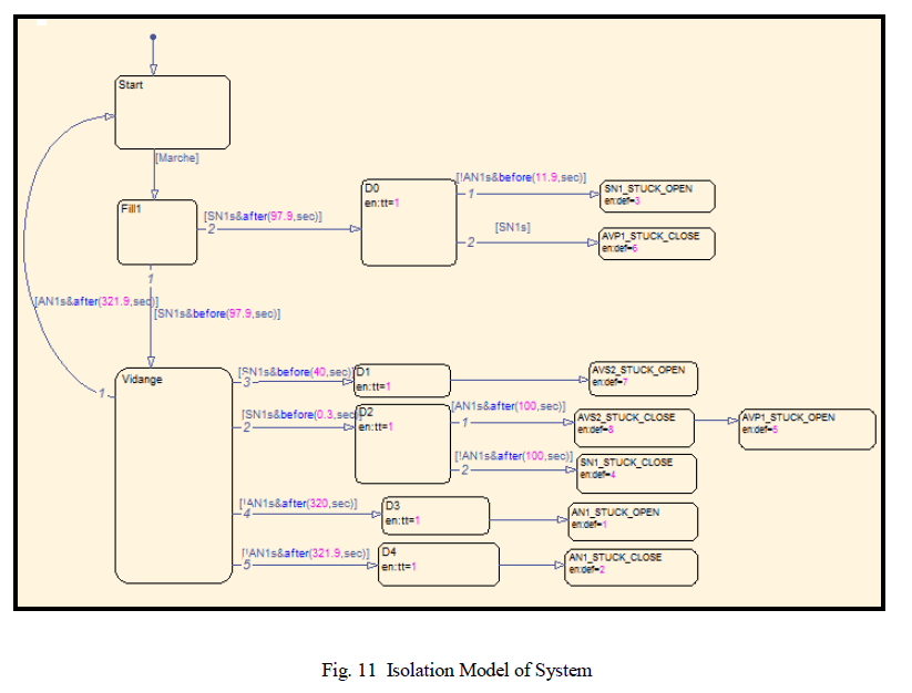
| The global automata graph for diagnosis of the two tanks system is shown in figure 10 (see Appendix B).If the modelof
the whole systemis built, the reading of theevolution of the systembecomes very difficult.Usingthe
tooltimedautomatonhasonly one drawbackis the explosionin the number oftransitions betweenstates inthe
threemodes.Thisexplosion probleminthe number of arcsis solved byusing thetoolstate flow (see Figure 11 in Appendix
C) |
SIMULATION RESULTS |
| To illustrate the effectiveness of the diagnosis approach, wepresent simulation results of the level regulation system
example. |
| The Bon graph and timed automata models of the system was constructed using MATLABSIMULINK and state flow.
Bond graph block and bloc program are developed by the authors which are not presentedin the paper |
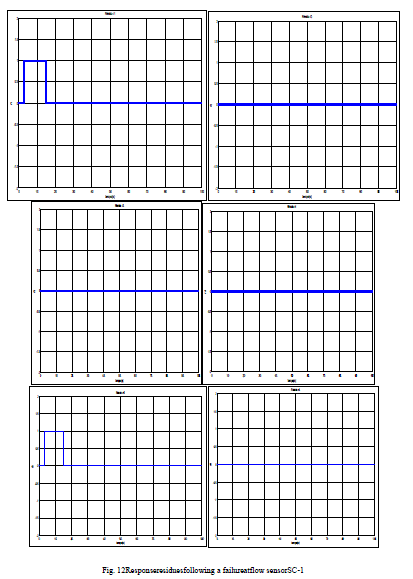
| Two failure scenarios were simulated. The first failure SC-flow sensor 1 during a time interval ranging from 3 to 15 s.
Figure 12 shows the response of r1 and r5 residues and their sensitivity to this failure. Referring to the signature component SC-1 (flow sensor) given in Table III shows that this result is consistent with what is planned, ie in case of
component failure SC-1 (flow sensor) only the residues r1 and r5 exceed their respective thresholds. |
 |
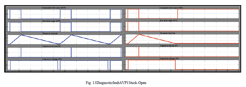 |
| Figure 13 enables us to comparenormal operation (left) of the process witha state offailedoperation(right).
Onthe right figure, despite the application to opentheAVP1valveremains closed. This time represents theoccurrence of
a failure. Toccurence=601.9sec. |
| Then,thesensorSN1,remains in stateS0,97.9secafterthe request to opentheAVP1valve.This momentisthe moment offault
detection. Tdétection=699.8sec. S0state. |
| FinallyAN1sensorremainsat 0, 20 seconds afteractivation of thedetection state. This momentcorresponds to thefault
location. Tlocalisation=719.8sec. |
| Thisfigure analysisshows that: |
| • Detection time=Tdétection-Toccurence=97.9sec. |
| • Localization time=Tlocalization–Tdétection=20 sec |
CONCLUSION |
| In this paper, a method for fault detection and isolation ispresented. It is combining graphical approaches (BG) and the
model of dynamical system (timedautomata). Bond graph is used for detecting systematically actuators; sensor and
structural fault.Also the fault isolation procedure based backward timeanalysis was presented. The localization
algorithm is used when the faults can not identify from the model of Bond Graph. |
| This isolation approach is based on trajectory and temporaltransition of the model must be identified for allconsidered
modes (faultless and faulty modes). Thetime of occurrence of fault is considered. The backward time analysis searches
the possible reversepath to localize the fault according the time of faultoccurrence.
Thenext stepis interestedin the eventoffault diagnosisin the presence ofcommon causes. |
ACKNOWLEDGMENT |
| The authors would like to thank the editor and refereesfor their insightful comments that greatly improved thecontent of
this paper. |
References |
- J. J. Gertler; âÃâ¬ÃÅFault detection and diagnosis in Engineering systemâÃâ¬ÃÂ, Ph. D. Dissertation, George Mason University, Fairfax, Virginia, 1998
- R. J. Patton; P. M. Frank and R.N. Clark, Issues in fault diagnosis for dynamic systemsâÃâ¬ÃÂ, Springer Verlag; New York, 2000.
- W. C. Hamascher, J. Decleeer and L. Console, âÃâ¬ÃÅreading in model based diagnosisâÃâ¬ÃÂ, Morgan-Kaufmann Pub, San mateo, 1992.
- R. Reiter,âÃâ¬ÃÂA theory of diagnosis from first principlesâÃâ¬ÃÂ, Artificial Intelligence, 1987, Vol. 32, pp. 55-95
- M. Staroswiecki and Comtet-Verga, âÃâ¬ÃÅAnalytical redundancy relations for fault detection and isolation in algebraic dynamic systemâÃâ¬ÃÂ, Automatica; 2000, pp. 111-120.
- B. Publido and C. Alonso-Gonzlez, âÃâ¬ÃÅAn alternative approach to dependency-recording engines in consistency-based diagnosisâÃâ¬Ã , Artificial Intelligence; 2000, pp. 111-120.
- B. Publido and C. Alonso-Gonzlez, âÃâ¬ÃÅAcompilation technique for consistency-based diagnosisâÃâ¬Ã , IEEE Tran, 2004, pp. 2192-2206.
- P. J/ Mosterman and G. Biswas,âÃâ¬ÃÂDiagnosis of continuous valued system in transient operating regionsâÃâ¬ÃÂ, IEEE trans, 1999, pp. 554-565.
- E. J. Manders, S. Narasimhan, G. Biswas and P. J. Mosterman, âÃâ¬ÃÅA combined qualitive/quatitative approach for fault isolation in continuous dynamic systemsâÃâ¬ÃÂ, IFAC, 2000, pp. 1074-1079
- F. E. Cellier âÃâ¬ÃÅContinuous System ModelingâÃâ¬ÃÂ, Springer Verlag, New York, 1991, pp.251-287.
- Dean C. Karnopp, Donald L. Margolis, Ronald C. Rosenberg, âÃâ¬ÃÅSystem dynamics: Modeling and simulation of mechatronic systemsâÃâ¬ÃÂ, 3rd ed., Wiley Interscience, New York, 2000, pp. 297-336.
- Z. Simeu-Abazi an all,âÃâ¬ÃÂBackward time analysis for the diagnosis of discrete event systemsâÃâ¬ÃÂ, Advanced Maintenance Engineering, Volume 1, Part 1, pp. 128-133.
- H. M; Paynter,âÃâ¬ÃÂAnalysis and design of engineering systemsâÃâ¬ÃÂ, MIT Press, Cambridge, 1961
- D. C. Karnopp and R. C. Rosenberg,âÃâ¬ÃÂSystem Dynamics: A unified ApproachâÃâ¬ÃÂ, John Wiley, New York, 1974
- Jean U. Thoma,âÃâ¬ÃÂSimulation by Bondgraphs âÃâ¬Ãâ Introduction to a graphical methodâÃâ¬ÃÂ, Springer-Verlag, New York, 1989.
- P. C. Breedveld,âÃâ¬ÃÂA systematic method to derive bond graph modelsâÃâ¬ÃÂ, Int Journal of modeling and simulation,1 (1), 57-62, 1986.
- A. Samantaray, K. Medjaher, B. OuldBouamama, M. Staroswiecki and G. Dauphin-Tanguy, Diagnostic bond graphs for online fault detection and isolation. . Simulation Modelling Practice and Theory, vol. 14(3), pp. 237âÃâ¬Ãâ262, 2006.
- R. El Harabi, B. OuldBouamama, M. El Koni Ben Gayed and M. Abelkrim, Bond graphs for diagnosis of chemical processes. Computers, chemical engineering, vol. 36, pp. 301âÃâ¬Ãâ324, 2012.
- Sava. A.T. Sur la synthese de la commande des systÃÆèmes ÃÆàÃÆévÃÆènementsdiscretstemporises. PhDthesis, LaboratoiredâÃâ¬Ãâ¢Automatique de Grenoble, Novembre2001.
- Simeu-Abazi Z., Rayhane H., Bennani T., Bouredji. Z. Optimisation des temps de detection dans la surveillance des systemes, 5eme Congres International de Genie Industriel, 25-29 Octobre 2003.
- OuldBouamama B., Medjaher K., BayartM.,Samantaray A.K., Conrard B.âÃâ¬Ã Fault detection and isolation of smart actuators using bond graphs and externalmodelsâÃâ¬ÃÂ. Control Engineering Practice, vol. 13, pp. 159âÃâ¬Ãâ175, 2005.
- OuldBouamama B., Medjaher K., Samantaray A.K., StaroswieckiM.âÃâ¬ÃÂSupervision of an industrial steamgenerator. Part I: Bond graph modelingâÃâ¬ÃÂ, Control Engineering Practice, vol. 14, pp. 71âÃâ¬Ãâ83, 2006.
- OuldBouamama B., Samantaray A.K., Staroswiecki M., Dauphin-Tanguy G.âÃâ¬ÃÂDerivation of constraint relations from bond graph models for fault detection andisolation Ãâû, in: Proc. ICBGMâÃâ¬Ãâ¢03, Simulation Series, vol. 35, nÃâð. 2, pp. 104âÃâ¬Ãâ109,ISBN: 1-56555-257-1, 2003.
|
Appendix |
 |
| B) Diagnosis Timed Automata Model |
 |
| C) Isolation Model constructed with state flow |
 |