Keywords
|
| Inverse control, reference model, neural networks, fuzzy logic, fuzzy clustering, nonlinear system, conical tank |
INTRODUCTION
|
| A basic problem in process industries is to control of liquid level and the flow in tanks. Conical tanks find wide applications in such industries, and they have been used by many authors in control literature for performance testing of control systems. The conical tank with gravity flow presents a strong nonlinearity because the extreme changes in area. |
| We propose, in this paper, a model reference direct inverse control strategy based on linear local models. In contrast to other works, the plant to be controlled is approximated by using Takagi-Sugeno fuzzy models. We demonstrate that the proposed control strategy is robust and simple. As shown in comparisons against other published papers, the setpoints of the process are reached fast and without overshoots. |
| The paper is organized as follows. Section II introduces the related work based on state-of-the-art of liquid level control for conical tanks. In Section III the parameters of the conical tank and the differential equation that defines its nonlinear mathematical model is introduced. Section IV explains in detail the proposed modeled of the tank. In order to obtain the TS fuzzy model, first we describe the TS fuzzy model and then the Fuzzy Clustering Algorithm. Also, in this section, we explain the identification stage and how we measure the accuracy of the model identified by means of the validation process. Section IV follows with the identification of two tanks showing the results obtained. In Section V we expose the theory about the Model Reference Direct Inverse Control. We begin this section with the inversion concept and its realizability and then we show the general structure to control a plant with reference model. To finish this section, we explain our proposal to implement the controller. In Section VI, we present two examples of design of level liquid control of two conical tanks and we compare and analyze the results obtained by our methodology with others control strategies applied to theses two cases. Finally, Section VII makes concluding remarks. |
RELATED WORK
|
| Because the level process of a conical tank has nonlinear characteristics, normally the plant is represented as a piecewise linearized model for a number of operating points. So, the process is identified through a number of transfer functions of First Order Plus Time Delay (FOPTD) representing an approximation to the real system [1]. From this viewpoint, the control is focused on FOPTD plants, also called First Order Plus Dead Time plants (FOPDT) [2]. In [3], the authors identified four first order transfer functions, with zero dead time, in four operating points, by process reaction curve method [4]. They propose a Proportional Integral (PI) controller [4] for each transfer function by using Direct Synthesis method [5] and Skogestad's method [6]. The results obtained showed the better behavior of Direct Synthesis method. |
| In addition, by using the process reaction curve method, a continuously tuned adaptive [7] PI controller according to the tank operating point is designed in [8]. The authors identified five FOPTD models, for five operating points. The estimated model parameters are used to calculate the controller based on the controller parameters and its operating points, and a tuning system was created. A comparison with a conventional PI, tuned by the Ziegler-Nichols (ZN-PI) rules [9], was performed and the results showed better performance of the adaptive PI controller. |
| In [10] a system identification using the process reaction curve method, to obtain four FOPTD models for four operative points, is introduced. The authors proposed the design of a Fuzzy Controller (FC) [11] and it is compared with a Proportional Integral Derivative (PID) controller [4]. The PID controller is based on Chien and Fruehauf proposal [12] that is an Internal Model Controller (IMC) based technique [13]. Results in [10] demonstrate the best performances of the FC. |
| A Fuzzy PI (FPI) controller [14] is proposed in [15] and compared with a ZN-PI controller. Results demonstrate the superior performance of the FPI controller. The design of the controllers is based on the linearized model in an operating point. |
| Genetic Algorithms (GA) [16] are used in [17] to design a PID, an IMC and a Transfer Function based controller. Three FOPTD transfer functions are identified by process reaction curve method. The performance of proposed controllers are compared against controllers tuned using ZN methods. The best controller was the IMC tuned by a GA. |
| More control techniques have been applied to control a conical tank. Thus, in [18] a Model Predictive Control (MPC) [13] has been applied and compared against a PID controller tuned by IMC technique. As in the previous cases, a FOPTD model was identified to design the two controllers. MPC gives better performances than PID controller. |
| In [19] a MPC, tuned by Sridhar and Cooper method [20], is proposed and compared against a PI controller based on Skogestad’s settings. The tank is approximated to a FOPTD model. It was observed that MPC shows a better tracking capability than a PI controller. |
| A GA also is used to tune the membership functions of the input variables of a Mamdani type FC [21] in [22]. The results of the FC are compared with a PI to evaluate its performances. The PI controller is designed using IMC technique. The results obtained show that FC performs better than PI controller. |
| Use of Soft Computing (SC) [23] is an alternative to control nonlinear systems. Thus, in [24] a FC, a FPI controller and a GA tuned controller are designed. A PI, tuned according to Skogestad’s method, is used as comparison. The results demonstrated that the controllers designed using SC techniques work better than the PI controller. |
| In [25] a ZN-PI controller is compared with a Particle Swarm Optimization [26] based PI (PSO-PI) controller [27] and with a Fractional Order PI (FO-PI) controller [28]. From the analysis, the proposed PSO-PI controller and FO-PI controller gives better performance compared to ZN-PI controller. |
| Two linear Generalized Predictive Controllers ([29], [30]) are designed and are compared in [31]. Also in [31] a Direct Inverse Control (DIC) [32] is introduced. This DIC was implemented by a neural network [33]. According to the results, they demonstrate the best behavior provided by the DIC. |
| In [34] a Time Optimal Control (TOC) system [35] and an Adaptive Control (AC) using neural networks are proposed. TOC is used to setpoint changes and AC is designed for the process parameters variations. Performance is compared with a PID tuned by ZN rules using process reaction curve method for six regions. The results prove the effectiveness of the TOC and AC. |
| As described previously, most of the authors make an approximation of the process through a number of transfer functions of First Order Plus Time Delay and then they apply some control technique. In this work, we make an approximate by mean of linear local models which have been obtained of a Takagi-Sugeno (TS) fuzzy model. Once the Takagi-Sugeno model is obtained, we apply the Model Reference Direct Inverse Control technique to control the liquid level in a conical tank. In [31], the authors apply the inverse control technique, but without to do an approximation of the model and training a neural network like the exact inverse. However, the controller obtained in [31] is more complex than our proposal although the results obtained are similars. |
MATHEMATICAL MODEL OF A CONICAL TANK
|
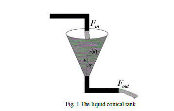
| Fig. 1 ilustrates the geometry relationship of the conical tank under study. As is shown, the shape is a cone and therefore the geometrical relationship is nonlinear. Conical tank parameters are: inflow rate (Fin ), outflow rate (Fout ), top radius (R ) and total height (H ). The control goal is to keep up the level (h ) of liquid at a constant value and for it we have to control the inflow rate. The radius of the cone is r for the level . The outflow rate is due to the hydrostatic pressure and it is not controlled. |
| For the level h the liquid volume is given by: |
 |
| Volume variation is the difference between the inflow and the outflow and it depends on the discharge coefficient kout , as follows: |
 |
| By differentiating the equation (1), then: |
 |
| Equalling (2) and (3): |
 |
 |
TAKAGI-SUGENO FUZZY MODEL OF THE PLANT
|
| Because the strong nonlinearity of the system under study, the plant is represented by a number of linear models. Thus the output of a model is calculated as an interpolation of locally linear models. The local linear models follow a TS fuzzy model. The fuzzy models are obtained by the Fuzzy Clustering Algorithm. |
| A. Takagi-Sugeno Model |
| The Takagi-Sugeno fuzzy model ([36], [37]), of a nonlinear dynamic system, interpolates local linear LTI (Linear Time Invariant) ARX (AutoRegressive with eXogenous input) models, as follows: |
 |
 |
 |
| B. Fuzzy Clustering Algorithm |
| The plant identification [38] consists obtaining a mathematical model applying test signals to the plant. The mathematical model is obtained by applying any identification algorithm, however, the complexity of the obtained model depends on the identification methodology. We use the fuzzy clustering algorithm as an identification algorithm in order to obtain the TS model. |
| Fuzzy Clustering Algorithms ([39], [40]) are best suited for fuzzy identification. Fuzzy C-Means (FCM) method [20] and the Gustafson-Kessel (GK) method [23] are the most used. Fuzzy clustering analytical techniques are based on the optimization (minimization) of the objective function c-means (Equation 6): |
 |
 |
| The major disadvantage of the FCM algorithm is that the obtained classes have hyper-ellipsoidal form. For control applications it is desirable that those classes have a linear form. |
| An alternative to FCM is the GK algorithm [41] that is adaptive with the distance. That is, the B matrix in (6) is different for each class (Bi). However, the objective function (6) cannot be directly minimized with respect to Bi, since it is linear in Bi. To obtain a feasible solution, Bi must be constrained in some way. The usual way is to constrain the determinant of Bi: |
 |
| Using the Lagrange multiplier method, the expression for Bi is obtained: |
 |
| where Fi is the fuzzy covariance matrix of the th cluster defined by: |
 |
| This algorithm detects quasi-linear behaviors quite well. However, the standard GK clustering algorithm presents numerical problems when the number of data samples is small or when the data within a cluster are linearly correlated. In such a case, the fuzzy covariance matrix Fi (9) cannot be inverted to calculate the norm-inducing matrix Bi (8), because Fi may become singular. Babuška ([42], [43]) proposed a solution to this problem applying a technique to calculate of the fuzzy covariance matrix. However, as a result one can get clusters that have little relationship with the real distribution of the data and consequently one obtains a poor TS fuzzy model. This problem occurs mainly when the number of data points in a cluster becomes too low. Babuška ([42], [43]) proposed a solution to this problem too, resulting a modified GK algorithm. |
| We use in this work the Fuzzy Modeling and Identification Toolbox (FMIT) developed by Babuška [44], that has been implemented the techniques for solving the problems of GK algorithm, i.e., the FMIT implements the modified GK algorithm. |
| C. Identification and Validation |
| For computing the height h, at each time instant, we use Simulink® [45]. The differential equation (4) and some variables inflows, Fin, functions are simulated for obtaining the height h in terms of time.. From the input (Fin) and the output (h) vectors and applying the FMIT we get the TS model. We use the half of the input samples in the identification process and the other half to the validation process. The validation process is used to calculate the identified model accuracy. For comparison between the computed output with the output of the plant we use the VAF (Variance Accounted For) index measurement, as follows: |
 |
 |
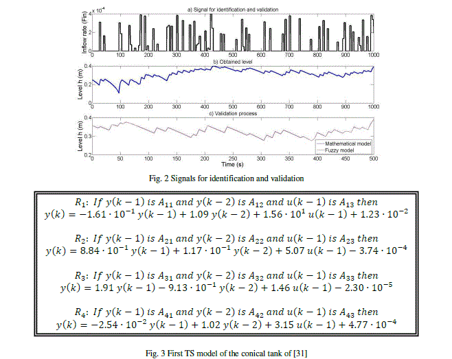 |
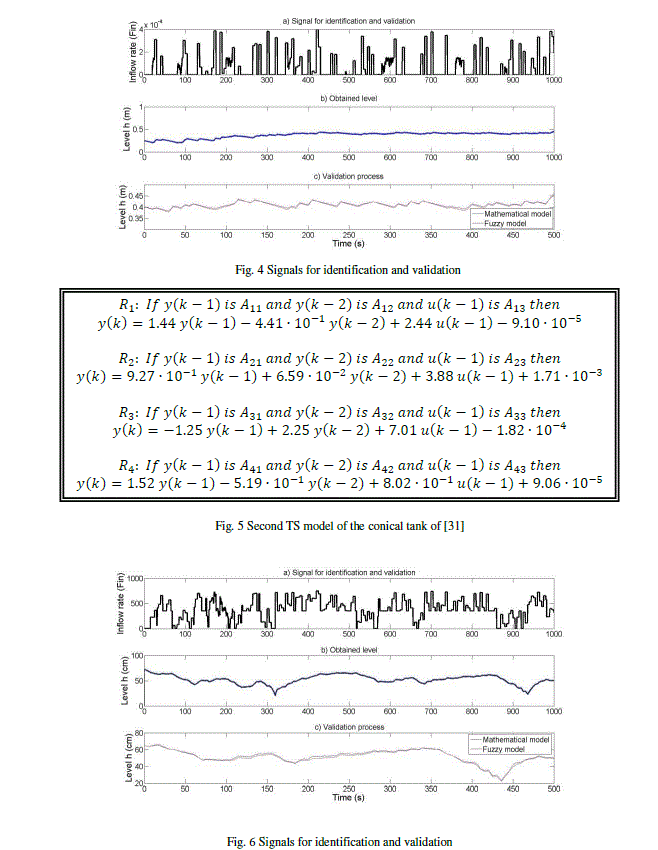
| A factor that determines the quality obtained in the mathematical model of the process is the choice of the used signals in system identification. To make a comparison with the obtained control, we have calculated other fuzzy model by adding a small random signal to the input (see Fig. 4), to ensure that the model will be able to accurately reproduce high frequency outputs of small magnitude. |
| In this case, we have obtained, with a fuzzification coefficient m = 2.51, a VAF = 96.3911, the TS model that is described in Fig. 5. |
| Although the second fuzzy model is less accuracy in the validation process, it gives best results in the subsequent quality control signal. |
 |
 |
 |
MODEL REFERENCE DIRECT INVERSE CONTROL
|
| The inverse model based control has made several appearances in the literature demonstrating its strength in improving parameters such as settling time, tracking and other performance metrics. In the Direct Inverse Control, the controller is a perfect inverse model of the plant. So, the plant output will equal to the reference signal. In the practice, however, it is impossible to get a perfect inverse. Furthermore, it is better to follow a smoothed version of the reference signal, like in the case of step reference. The smoothed version of the reference signal is the desired output of the controlled system and it is modeled by the reference model. The reference model is a filter and it is designed as a function of some parameters, such as the rising time, the settling time, maximum overshoot and steady-state error. |
A. Inversion Concept and Realizability
|
 |
 |
 |
B. Model Reference Control
|
| The idea of the reference model was due to Whitaker [47] and it consists in that the output of closed loop system is equal to the output of a reference model or similar to it. |
| Fig. 9 shows the general structure to control a plant with reference model. The controller attempts to make the output of the plant coincides with the output of the reference model in an asymptotic form. |
| The error at the output e(t), i.e. the difference between the output of the reference model yr(t) and the output of the plant y(t), depends on the error in obtaining the plant model (uncertainty), the variations in the output of the plant due to disturbance and the error in the model output representing the controller. |
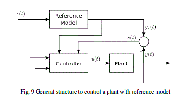 |
| The reference model, which should be of exponentially stable dynamic, is chosen to have the same dynamic response that to the designer would like for the controlled system. Therefor, the designer must have enough knowledge of the plant to define the desired behavior through the model. |
| C. Implementation of the controller |
| Fig. 10 shows the basic scheme of the system. The main aim is that the output of the plant, y(t), being equal to the output of the reference model, yr(t). Suppose the reference is as follows: |
 |
| Doing the Z inverse transform, the difference equation of the output of the reference model is: |
 |
 |
 |
 |
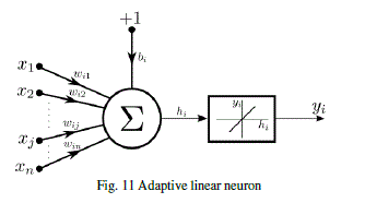
| The expression of the control signal in equation (13) is implemented by a neural network ([31], [33]). This neuron has weights Wij, bias bi and linear activation function, that is, the neuron is a ADAptive LInear NEuron (ADALINE), that was introduced by Widrow in 1959 (see Fig. 11). In general, a neuron generates an output given by: |
 |
| In equation (14), is the neuron number and is the input number. |
 |
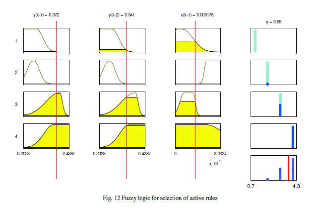
| The final system is a feedback system because the control signal in equation (13) depends on the output of the system. The number of rules of the TS fuzzy model will determine the number of neurons of the controller. Each neuron will have one output. We have designed a fuzzy logic which uses the antecedents of the rules. |
| Because the connective of the antecedent is the "and", it is necessary to active the three fuzzy sets to activate a rule. For example, to activate the rule R1 it is necessary that the fuzzy sets A11, A12 and A13 are activated. The designed fuzzy logic will generate a value in the deffuzification process indicating the active rules. For example, if only the rule R1 is activated, the fuzzy logic will give the value 1 and the control signal of the plant will be generated by that rule, i.e., only one neuron will generate the control signal. When more than one rule is activated, i.e., the rules R3 and R4 , the fuzzy logic will give a value between 3 and 4, for example 3.65 (see Fig. 12). It indicates that the rule R3 has 35% of weight in the control signal and the rule R4 has 65% of weight. Fig. 12 shows an example when two rules are activated simultaneously |
 |
DESIGN AND COMPARATIVE EXAMPLES
|
| In this section, the design of the control system for two conical tanks is illustrated. Comparisons against [31] and [3] demonstrate the advantages of the proposed approach. |
| A. Example 1 |
In [31], two linear Generalized Predictive Controllers (GPC) in two different linearized points are designed. Fig. 13 shows the response for the linearized GPC in the process point  and Fig. 14 shows the response for the linearized GPC in the other point and Fig. 14 shows the response for the linearized GPC in the other point  |
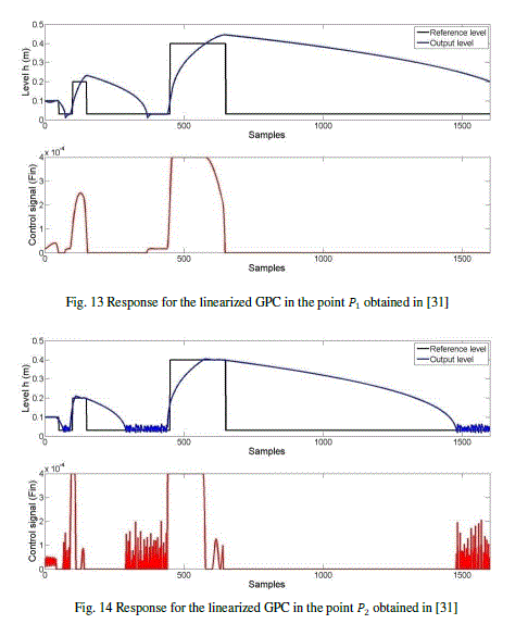 |
| Predictably, the first controller works well for small levels, while the latter performs better for larger levels. |
| Also in [31] is designed a Direct Inverse Control (DIC). The response obtained, as shown in Fig. 15, has a better behavior and it is as fast as, physically, is possible. When there is a change of setpoint, to fill up the tank, the control signal is maximum until nearly to get the desired height. Thus, the control signal type "bang-bang" has been ideal to control this tank. The design of this DIC, by trial and error method, was implemented by a neural network with seven hidden neurons. The network was trained by Levenberg-Marquardt algorithm with 500 iterations and the inverse model is used like a controller. |
| Now, we will see the results with our proposal by choosing a reference model equal to the equation (11). Fig. 16 shows the results for the TS model of Fig. 3. As is shown, to keep up stable the achieved levels, the control signal varies very fast and, in practice, this is a problem due to the speed of opening and closing of the valve that supplies the inflow. This variation of the control signal is because the designed system switches between two of the rules to maintain a constant level. |
| Fig. 17 illustrates the response of the TS model of Fig. 5. Here, the control signal is better and practically equal to that of Fig. 15. Here the control system uses only one rule to maintain a constant level and for it the control signal is constant. |
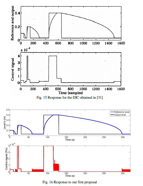 |
| An advantage of our method is that in [31] the architecture of the neural network by trial and error testing was obtained, while we obtained the architecture of the neural network from the identification phase. This means that we don’t need to test the architecture, to train it, and to check the results. Following our proposal, the architecture of the neural network is obtained without training and testing. Another advantage of our method is the reduction of the number of neurons, because our neural network uses four neurons against the seven of the DIC [31]. Thus, the hardware or software that implements the neural network will be simpler. |
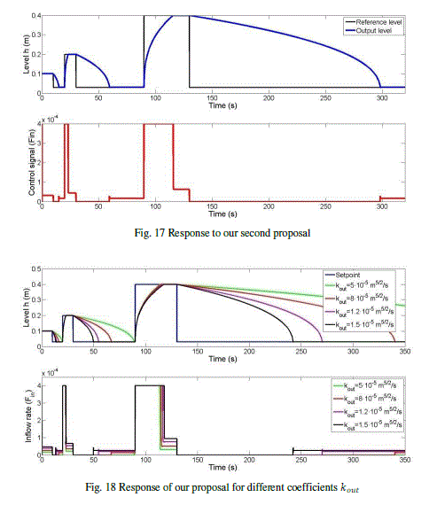
| Although in [31] a robustness study has not presented, we show in Fig. 18 that our system is robust against changes of Kout and the behavior of the control signal continues being ideal. |
 |
| B. Example 2 |
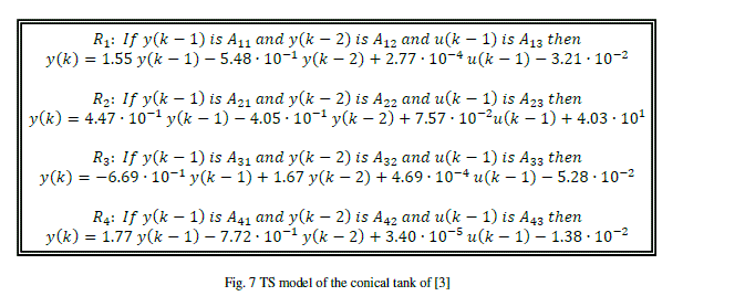
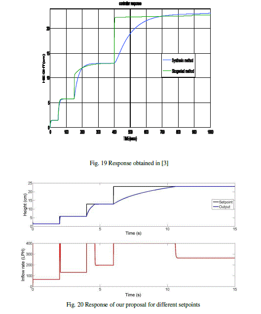
| In this second example, we use the conical tank controller introduced in [3]. The authors identified a first order model for four points: 1.44 cm, 5.76 cm, 12.83 cm and 23.04 cm of height. For each operating point, a PI controller was designed by the direct synthesis method and by the Skogestad's method. Fig. 19 shows the obtained results. |
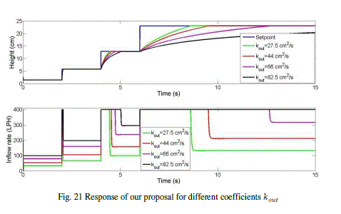
| Following our approach, and by applying the same method of the example 1, the controller is obtained from the model illustrated in Fig. 7. Fig. 20 shows the behavior of the proposed controller. |
| As is shown, our design has a much faster behavior because the controller uses the maximum inflow rate when there is a change of setpoint. However, the design made in [3], by Synthesis method and Skogestad’s method, do not use the maximum inflow rate and furthermore the inflow rate increases, progressively, and it is not of type “bang-bang” which is ideal for this type of application. |
| Table 1 summarizes the settling time in seconds, which is measured around the ±2% of the final value, for the graphs of Figures 19 and 20. |
| Fig. 21 demonstrates that our proposal is robust. In this case, we show that if we vary the coefficient kout around ±20% and ±50% the system is stable and only varies the filling up speed. The discharging coefficient is related with the stability of the system, while the rest of the parameters are kept almost constant. |
 |
 |
 |
CONCLUSION
|
| In this work, a new model reference direct inverse control strategy based on linear local models has been proposed. We approximate the process by using Takagi-Sugeno fuzzy modeling. The proposed approach is applied to liquid level and flow control of conical tanks. Despite conical tank control is a hard nonlinear problem, the obtained controller following the proposed approach results robust and its implementation simple in hardware. We demonstrate that the controller is robust against variation of the discharge coefficient kout up to ±50%. The controller implementation is built of four ADALINE neurons and a fuzzy logic for selecting those neurons that generate the control signal. The identification phase is offline, therefore the neural network is obtained without training and testing. As shown in comparisons against other published results, the setpoints of the process are reached as fast as possible without overshoots. |
| |
References
|
- Fedele, G., “A new method to estimate a first-order plus time delay model from step response”, Journal of the Franklin Institute, Vol. 346,Issue 1, pp. 1-9, 2009.
- Normey-Rico, J. E., Control of Dead-time Processes, Ed. Springer, 2007.
- Aravind, P., Valluvan, M., and Ranganathan, S., “Modelling and Simulation of Non Linear Tank”, International Journal of AdvancedResearch in Electrical, Electronics and Instrumentation Engineering, Vol. 2, Issue 2, pp. 842-849, 2013.
- Johnson, M. A., and Moradi, M. H., PID Control – New Identification and Design Methods, Ed. Springer-Verlag London Limited, 2005.
- Chen, D., and Seborg, D. E., “PI/PID Controller Design Based on Direct Synthesis and Disturbance Rejection”, Industrial &EngineeringChemistry Research, Vol. 41, Issue 19, pp. 4807-4822, 2002.
- Stogestad, S., “Probably the best simple PID tuning rules in the world”, Journal of Process Control, Vol. 13, Issue 4, pp. 291-309, 2003.
- Astrom, K. J., and Wittenmark, B., Adaptive Control, Second Edition, Ed. Dover Publications, 2008.
- Anand, S., Aswin, V., and Kumar, S. R., “Simple Tuned Adaptive PI Controller for Conical Tank”, International Conference on RecentAdvancements in Electrical, Electronics and Control Engineering, pp. 263-267, 2011.
- Ziegler, J. G., and Nichols, N. B., “Optimum settings for automatic controllers”, Transactions of the American Society of MechanicalEngineers, Vol. 64, pp. 759-768, 1942.
- Sowmya, P., Srivignesh, N., Sivakumaran, N., and Balasubramanian, G., “A Fuzzy Control Scheme for Nonlinear Process”, InternationalConference On Advances in Engineering, Science And Management, pp. 683-688, 2012.
- Grigorie, T. L., Fuzzy Controllers, Theory and Applications, Ed. Lucian Grigorie, Publisher InTech, 2011.
- Chien, I. L., and Fruehauf, P. S., “Consider IMC Tuning to Improve Controller Performance”, Chem. Eng. Progr., Vol. 86, pp. 33-41, 1990.
- Brosilow, C., and Joseph, B., Techniques of Model-Based Control, Ed. Prentice Hall PTR, 2002.
- Jantzen, J., “Tuning of Fuzzy PID Controllers”, Technical Univ. of Denmark: Dept. of Automation, Technical report 98-H 871, 1998.
- Anandanatarajan, R., Chidambaram, M., and Jayasingh, T., “Improved Design of FLC for a First Order Nonlinear Processes with Dead Time”,Proceedings of International Conference on Intelligent Sensing and Information Processing, pp. 466-471, 2004.
- Goldberg, D. E., Genetic Algorithms in Search, Optimization & Machine Learning, Ed. Pearson Education, 2013.
- Valarmathi, R., Theerthagiri, P. R., and Rakeshkumar, S., “Design and Analysis of Genetic Algorithm Based Controllers for Non LinearLiquid Tank System”, IEEE-International Conference On Advances In Engineering, Science And Management, pp. 616-620, 2012.
- Sukanya, R., and Sivanandam, V., “Design of Controllers based on MPC for a Conical Tank System”, International Conference On AdvancesIn Engineering, Science And Management, pp. 309-313, 2012.
- Venkatesan, N., and Anantharaman, N., “Controller design based on Model Predictive Control for a nonlinear process”, 8th InternationalSymposium on Mechatronics and its Applications, pp. 1-6, 2012.
- Shridhar, R., and Cooper, D., “A tuning strategy for unconstrained multivariable model predictive control”, Industrial &EngineeringChemistry Research, Vol. 37, Issue 10, pp. 4003-4016, 1998.
- Lilly, J. H., Fuzzy Control with Mamdani Systems, Ed. John Wiley & Sons, Inc., 2010.
- Madhubala, T. K., Boopathy, M., Sarat Chandra, J., and Radhukrishnan, T. K., “Development and Tuning of Fuzzy Controller for a ConicalLevel System”, Proceedings of International Conference on Intelligent Sensing and Information Processing, pp. 450-455, 2004.
- Chaturvedi, D. K., Soft Computing: Techniques and Its Applications in Electrical Engineering, Ed. Springer-Verlag Berlin Heidelberg, 2008.
- Nithya, S., Sivakumaran, N., Radhakrishnan, T. K., and Anantharaman, N., “Soft Computing Based Controllers Implementation for Non-linearProcess in Real Time”, Proceedings of the World Congress on Engineering and Computer Science, Vol. 2, 2010.
- Priya, C., and Lakshmi, P., “Fractional Order Controller Design and Particle Swarm Optimization Applied to a Nonlinear System”, IEEEInternationalConference on Recent Trends in Information Technology, pp. 959-964, 2011.
- Olsson, A. E., Particle Swarm Optimization: Theory, Techniques and Applications, Ed. Nova Science Publishers, Incorporated, 2011.
- Anantharaman, N., Dharmalingam, V., Giriraj, S. M., Radhakrishnan, T. K., and Sivasankar R., “Particle Swarm Optimization TechniqueBased Design of PI controller for a Real-Time Non-Linear Process”, Instrumentation Science and Technology, Vol. 36, Issue 5, pp. 525-542, 2008.
- Monje, C., Chen, Y., Vinagre, B., Xue, D., and Feliu, V., Fractional-order Systems and Controls, Ed. Springer: Advances in IndustrialControl, 2010.
- Clarke, D. W., Mohtadi, C., and Tuffs, P. S., “Generalized Predictive Control - Part I”, Automatica, Vol. 23, Issue 2, pp. 137-148, 1987.
- Clarke, D. W., Mohtadi, C., and Tuffs, P. S., “Generalized Predictive Control - Part II”, Automatica, Vol. 23, Issue 2, pp. 149-160, 1987.
- NØrgaard, M., Ravn, O., Poulsen, N. K., and Hansen, L. K., Neural Networks for Modelling and Control of Dynamic Systems, 3rd printing, Ed.Berlin, London: Springer-Verlag, 2003.
- Widrow, B., and Walach, E., Adaptive inverse control, IEEE Press, Ed. Wiley-Interscience, 2008.
- Yegnanarayana, B., Artificial Neural Networks, Ed. Prentice-Hall of India, 2006.
- Bhuvaneswari, N. S., Uma, G., and Rangaswamy, T. R., “Adaptive and Optimal Control of a Non-linear Process Using IntelligentControllers”, Applied Soft Computing, Vol. 9, Issue 1, pp. 182-190, 2009.
- Kirk, D. E., Optimal Control Theory: An Introduction, Ed. Dover Books on Electrical Engineering, 2004.
- Takagi, T., and Sugeno, M., “Fuzzy Identification of Systems and Its Applications to Modeling and Control”, IEEE Transactions on Systems,Man and Cybernetics, Vol. 15, Issue 1, pp. 116-132, 1985.
- Abonyi, J., Fuzzy Model Identification for Control, Ed. Publisher Birkhäuser Boston, 2003.
- Ljung, L., Systems Identification. Theory for the User, 2nd edition, Ed. Berlin, Prentice-Hall, 1999.
- Höppner, F., Klawonn, F., Kruse, R., and Runkler, T., Fuzzy Cluster Analysis. Methods for Classification, Data Analysis and ImageRecognition, Ed. John Wiley & Sons Ltd, 2000.
- De Oliveira, J. V., and Pedrycz, W., Advances in Fuzzy Clustering and its Applications, Ed. John Wiley & Sons Ltd, 2007.
- Gustafson, D. E., and Kessel, W. C., “Fuzzy Clustering with a Fuzzy Covariance Matrix”, Inproceeding of Decision and Control includingthe 17th Symposium on Adaptive Processes, IEEE Conference on, Vol. 17, pp. 761-766, 1978.
- Babuška, R., Fuzzy Modeling for Control, Ed. Kluwer Academic Publishers, Boston, 1998.
- Babuška, R., Van Der Veen, P. J., and Kaymak, U., “Improved Covariance Estimation forGustafson-Kessel Clustering”, Proceedings of the2002 IEEE International Conference on Fuzzy Systems, Vol. 2, pp. 1081-1085, 2002.
- Babuška, R., Fuzzy Modeling and Identification Toolbox, Cont. Eng. Laboratory, Faculty ofInformation Technology and Systems, 1998.
- “SIMULINK®, Dynamic System Simulation for MATLAB®,” The MATHWORKS Inc., 2013.
- Rigney, B., Pao, L., and Lawrence, D., “Nonminimum phase dynamic inversion for settle timeapplications”, IEEE Transactions on Control Systems Technology, Vol. 17, Issue 5, pp. 989-1005, 2009.
- Osburn, P., Whitaker, H., and Kezer, A., “New developments in the design of adaptive control systems”, 29th Annual Meeting, Institute ofAeronautical Science, No. 6139, 1961.
|