Research & Reviews: Journal of Material Sciences
ISSN:2321-6212
ISSN:2321-6212
Huang YC 1*, Yang WL2, Huang YC3
1Department of Electrical Engineering, National University of Tainan, Tainan, Taiwan
2Department of Computer Science and Information Engineering, National University of Tainan, Tainan, Taiwan
3Department of Materials Science and Engineering, National Yang Ming Chiao Tung University, Hsinchu, Taiwan
Received: 08-Mar-2023, Manuscript No. JOMS-23-91099; Editor assigned: 10-Mar-2023, PreQC No. JOMS-23-91099 (PQ); Reviewed: 24-Mar-2023, QC No. JOMS-23-91099; Revised: 31-Mar-2023, Manuscript No. JOMS-23-91099 (R); Published: 10-Apr-2023, DOI: 10.4172/2321-6212.11.2.003.
Citation: Huang YC. Efficient Pressure Sensors Placement for Water Distribution Network Using Flow-Tracking Analysis. RRJ Mater Sci. 2023;11:003.
Copyright: © 2023 Huang YC. This is an open-access article distributed under the terms of the Creative Commons Attribution License, which permits unrestricted use, distribution, and reproduction in any medium, provided the original author and source are credited.
Visit for more related articles at Research & Reviews: Journal of Material Sciences
This study presents a novel approach for efficient placement of top pressure sensors in water distribution network. Flow-Tracking Analysis using the head loss coverage ratio explores the least number of top sensors in network topologies. The following sequence of top sensor plans can be effortlessly determined by a simple greedy algorithm. A regular hydraulic model with 33 sensor nodes is adopted to validate the fast and effective feature of flow-tracking analysis. A top set of 5 sensor nodes selected by the head loss coverage ratio Hcr in flow-tracking analysis agree exactly with top set of 5 sensitive nodes selected by the objective function of sensitivity f(Xk) by means of sensitivity analysis. A linear relationship between the objective function of sensitivity f(Xk) and the head loss coverage ratio Hcr of top sensor nodes reveals high accuracy mapping from flow-tracking analysis to sensitivity analysis. Time complexity of searching top sensors node set by means of flow-tracking analysis is O(m✕(n+p)), contrasting starkly with the one in sensitivity analysis, O(Cnm). The average pressure error can be expected as low as 0.08 m with top-two sensors in sensors layout. As top sensors in the placement plan are all used, a minimum error of 0.04 m is achieved. Notably, Flow-Tracking Analysis has the advantages of less time complexity and accurate top sensors strategy as a new efficient solution for pressure sensors placement in the associated flow network.
Flow-tracking analysis; Pressure sensors; Water distribution network; Hydraulic models; Flow resistance; Fluid dynamics
Pressure monitoring plays a crucial role in resources management of urban Water Distribution Network (WDN). Pressure sensors should be located in least places where they can offer most valuable monitored data in WDN. It is unfeasible to install pressure sensors all around the network, but efficient placement of pressure sensors using hydraulic models may assist performance insufficiency of network operation and become a viable alternative.
As a project buried underground, WDN is complicated because it is composed of hundreds of thousands of pipes, junctions, pumps, valves, and storage tanks [1]. Thus, a hydraulic modelling (e.g. EPANET) is required as a simulation to have a comprehensive grasp on flow patterns and pressure variations of distributed network [2]. WDN modelling requires parameters such as water consumption, valve open/closed status, and pipe roughness, etc.
Water consumption and the status of valve opening/closing vary with daily life and operating conditions of water supply. Such variables can only be monitored by instruments or mathematical predictions. However, the roughness of pipes, which represents the flow resistance of pipes and fittings in the network, is a parameter that does not change for a period of time [3,4]. Moreover, pipe roughness is an important parameter for simulating the pressure distribution of the network. Therefore, the calibration of the pipe roughness coefficient is essential for the application of the hydraulic model [5]. To calibrate the pipe roughness coefficient, the first step is to estimate the initial value of each pipe. Then one should compare the simulated pressure values from the hydraulic model with the values from measurement [6-8].
How to select the pressure sensor nodes in a water distribution network is critical for pipe roughness calibration. Schaetzen, et al. presented three methods to select pressure sensor nodes to calibrate pipe roughness coefficients, one of which ranks the sampling locations based on shortest path algorithms [9]. Klapcsik, et al. discussed two approaches to the problem of locating the top pressure sensor nodes in a hydraulic system [10].
One of them applies the concept borrowed from graph theory to optimize the pressure measurement locations, whereas the other applies the sensitivity analysis of the pipe roughness affecting the node pressure. However, the above methods lack the physical basis for the fluid dynamics of water supply. Yoo, et al. developed a method considering the pipe connectivity of water distributed network and the impact among nodes by pressure-driven analysis and entropy method [11]. Lee, et al. defined a concept of coverage and proposed methods on how to locate monitoring sites by analysing the pathways of water flows in a designated water network [12].
Even though Yoo and Lee’s works are related to the physical properties of the pipe network, both do not grasp the pressure change of the entire loop from the water source to the pressure sensor node.
This study proposes a new approach, based on the coverage concept of head loss in flow tree diagram, to select the top set of locations for pressure sensors placement efficiently. According to the energy conservation law of fluid dynamics, their relationships are developed by means of flow tracking analysis from water source to pressure sensor node. Sequence configuration for this selected top group of sensor nodes is easily constructed by the greedy algorithm, and hence is able to greatly improve the computational efficiency.
Flow-tracking analysis
Water head refers to the pressure of piped water at the node (expressed in meters), plus the elevation of the node (expressed in meters). Therefore, the unit of pressure and water head used in this paper is meter. For convenience, the term pressure can replace water head if the elevation of the node is zero.
The head loss of pipe is the pressure drop caused by the surface friction inside the pipe. Head loss in the pipe can be calculated using the Hazen-Williams formula, which is often known as an empirical equation for evaluation of pressure drop in water distribution networks [2]. head Loss (hL) is determined by flow rate (q), pipe roughness coefficient (C), pipe diameter (d), and pipe length (L), as expressed in the following Hazen-Williams equation:
hL=A q1.852…….. 1
where
A=4.727 C-1.852 d-4.871 L
A network W(R, V, E) is shown in Figure 1, where R is the set of water sources, V is the set of nodes and E is the set of edges (or pipes) in the network. The water head (or pressure) at the node i ∈ V, can be calculated by the following hydraulic model formula

Figure 1. A typical hydraulic model W (2, 33, 50) with flow direction.
Pi=f (HRj, HLk) …….. 2
where Pi is the simulated pressure at ith node, 1 ≤ i ≤ |V|. |V| is the number of nodes. HRj is the set of all water heads (or pressures) of water sources, 1 ≤ j ≤ |R|, and HLk is the set of all head losses of the pipes, 1 ≤ k ≤ |E|. |R| and |A| are the number of water sources and the number of pipes, respectively. Note that we can compute the head loss hL for all the pipes if HRj is known and Ck represents the roughness coefficient of kth pipe in Equation 2.
As a result, the pressure at each node Pi is obtained by Equation 2, 1 ≤ i ≤ |V|. In the practical network operations, it is often assumed that the values of q, d, and L in Equation 1 are given. Hence, the problem of given HLk set is corresponding to the problem of getting appropriate Ck, where Ck is the set of all pipe roughness coefficients, 1 ≤ k ≤ |E|. To avoid random speculation of HLk, a node subset U (U ⊆ V, |U|=m), installed with pressure sensors, is necessary. A typical hydraulic model with two water sources, 33 nodes, and 50 pipes was adopted as shown in Figure 1.
All node elevations are set to be zero for simplicity. The red lines denote the main pipes with a diameter of 200 mm. The diameter of the other pipes is 100 mm, and the length of each pipe is 1000 m. All nodal demands are set to be 4.0 m3/h and the supply pressure head of both water sources is 35 m.
According to Equation 1, the roughness coefficient can be calculated from the head loss when the pipe diameter, pipe length and flow rate are given. Since WDN has numerous nodes, how to locate pressure sensors at a limited number of nodes efficiently and calibrate the pipe roughness coefficient accurately is the primary concern of this study.
The concept of calibration-weighting has to present in the process of selecting locations of pressure sensors. When a pressure sensor node is selected, the roughness coefficient of some pipes can be calibrated by Equation 1, while other pipes cannot. Several methods for optimal locations of pressure sensors in earlier works were introduced. The following will describe in detail how to use Flow-Tracking Analysis (FTA) to find optimal sensor nodes. According to the theory of fluid dynamics, this study proposes the head loss coverage ratio to quantify the concept of calibration-weighting. Head-loss coverage ratio Hcr is defined as
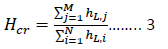
where N and M are the total number of pipes in the network and on the flow-tracks of the pressure sensor nodes, respectively. hL,j and hL,i represents the head loss of the jth pipe in those flow-tracks and of the ith pipe in the network, respectively. Hcr is a fraction of head loss coverage desired to be unity.
Figure 2 shows a typical two branches on the water distribution system with three end nodes of N5, N6, and N11. All pipes in Figure 2 have same roughness coefficient, diameter, and length. However, if merely two pressure sensors can be installed, options N5-N11 and N6-N11 are better than N5-N6, since the first two options can cover more pipes than the third option does. More specifically, the Hcr of N6-N11 is 0.994 higher than that of N5-N6, 0.739. This means that N6-N11 is preferred to N5-N6 mostly because N11 is a major end node as mentioned above. Therefore, this study will begin a procedure by evaluating Hcr as the index of priority rank in the greedy algorithm as follows.

Figure 2. Flow-Tracking of end nodes in two branches in the water distribution system.
Steps 1-7 are FTA and greedy algorithm proceeds as described:
1. Calculate flow directions of all pipes with EPANET. The pipe connects two nodes, and water flows from the upstream node to the downstream node.
2. Search for nodes where water can only flow into but not out. These sensor nodes are candidates for installing pressure sensors.
3. Calculate Hcr for each sensor node.
4. Sort all the Hcr values in a descending order.
5. The node with the largest Hcr is the first priority sensor node.
6. In addition to the maximum Hcr, select another sensor node among the other sensor nodes, so that the combination Hcr of the two nodes is maximized. This is the second priority sensor node.
7. With the same routine as step 6, the third, fourth, and until the last priority sensors all get into positions.
5 top sensor nodes in Figure 3 are determined according to step 2. The flow-tracking of node 21 is shown in Figure 4. The Hcr of node 21 is calculated from pipes with red colour. The Hcr of five sensor nodes is shown in Table 1. Column I in Table 1 is the sensor nodes sorted by Hcr in a descending order. Table 1 is the result of FTA. The next stage is continued by greedy algorithm. Since node 28 is the first priority, all combinations of the other nodes with node 28 are shown in column III in Table 2. Since Hcr of node 28 and 30 is the highest in column IV, node 30 is the second priority of the list. It can be seen from Table 1 that Hcr of node 16 is ranked second, but its jointed result with node 28 is far inferior to the jointed result of node 30 and node 28. After greedy algorithm, node 16’s final selection ranking fell to fifth. The reason is obvious from Figure 5 that nodes 16 and 28 only differ in one pipe (pipe 48).

Figure 3. Five optimal sensor nodes marked as red circle.

Figure 4. Flow-Tracking red tree diagram of node 21.
| Node | Hcr | FTA rank |
|---|---|---|
| 28 | 0.758 | 1 |
| 16 | 0.632 | 5 |
| 21 | 0.373 | 3 |
| 32 | 0.297 | 4 |
| 30 | 0.271 | 2 |
Table 1: Hcr and FTA rank of optimal sensor nodes by FTA.
| 1st node | Hcr | 1st-2nd nodes | Hcr | 1st-2nd-3rd nodes | Hcr | 1st-2nd-3rd-4th nodes | Hcr | 1st-2nd-3rd-4th-5th nodes | Hcr |
|---|---|---|---|---|---|---|---|---|---|
| 28 | 0.758 | 28-30 | 0.863 | 28-30-21 | 0.962 | 28-30-21-32 | 0.989 | 28-30-21-32-16 | 1 |
| 16 | 0.632 | 28-21 | 0.857 | 28-30-32 | 0.89 | 28-30-21-16 | 0.973 | ||
| 21 | 0.373 | 28-32 | 0.8 | 28-30-16 | 0.874 | ||||
| 32 | 0.297 | 28-16 | 0.769 | ||||||
| 30 | 0.271 |
Table 2: Rank of grouped sensor nodes by greedy algorithm.

Figure 5. Flow-Tracking red tree diagram of node 28 and 16.
High compatibility with sensitivity analysis
FTA finds pressure sensors placement by the concept of head loss based on fluid dynamics; Sensitivity Analysis (SA), however, employs an intuitive method to search the most sensitive pressure sensor point [9,10]. To search the best combination of k sensor nodes, an objective function of sensitivity f(Xk) as indicated by Equation 4 is proposed by Klapcsik, et al.
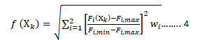
where wi is the weight of F1(Xk) and F2(Xk), F2,max=ln (N) and N is the total number of pipes. The objective is to define the sampling set that has the minimum values of Equation 1. It appears that FTA and SA use different strategy with critical index such as Hcr and f(Xk) for selecting the sensor nodes. However, no matter which possible order among the optimal set would be, optimal set of sensor nodes by both FTA and SA are precisely the same (Table 3). In order to verify this unique relationship, f(Xk) in Table 3 shows an excellent matching in each possible combination. FTA demonstrates a great agreement and perfect link directly to SA.
The head loss coverage ratio has exponential power sensitivity to the roughness coefficient, as in Equation 4. In other words, the head loss coverage ratio Hcr and the objective function of sensitivity f(Xk) reach one goal. Notably, f(Xk) is a search strategy function in SA and Hcr is the flow-tracking index behind search strategy of FTA. Figure 6 reveals a linear correlation between f(Xk) and Hcr in the optimal combination of top sensors. The correlation coefficient r closes to -1, indicating that a perfect linear relationship is found.

Figure 6. A perfect linear correlation between f(Xk) and Hcr in the best combination of optimal sensors.
The difference in solving pressure sensor placement problems from theory or phenomenon is their efficiency. Equation 5 expresses time complexity of SA as the number of combinations of m sensor nodes selected from n network nodes.

Time complexity regarding an algorithm is generally expressed in terms of a big O notation, which describes operation time taken to run an algorithm for performance evaluation. Equation 6 is the time complexity of FTA.

where n is the number of all nodes, m is the number of sensors and p is the number of all pipes. Because SA lacks the guidance of fluid dynamics to select sensor nodes, it can only choose randomly and compare the value of Equation 4.
The ratio of time complexity in choosing optimal 5 sensor nodes out of 33 nodes and 50 pipes by Equation 6 of FTA to Equation 5 of SA is

The average pressure simulation error Perr will improve reliability.
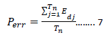
where Edj is pressure error of the jth test and Tn is the total test number set to 100 in this paper. The Perr of the top-ranked combination in the optimal set is shown in Table 3. Perr less than 0.1 m can satisfy the error requirement of the hydraulic model calibration. In this case, FTA needs two sensor nodes 28 and 30 for the model verification.
In the future, moreover, FTA can make the work of pressure sensor placement in massive water distribution network much easier by partitioning WDN into several smaller sub-networks. Then pressure sensor placement in sub-networks can be resolved one by one with the FTA algorithm. Optimal sensors node set in each sub-network can be integrated, and successive execution using FTA becomes faster and simpler. The resulting placement process for pressure sensors in enormously complicated WDN by means of FTA saves more time and work. Consequently, FTA characterized by fast and low time complexity is especially valuable to offer optimal top sensors set of the placement layout efficiently and cost-effectively.