ISSN ONLINE(2320-9801) PRINT (2320-9798)
ISSN ONLINE(2320-9801) PRINT (2320-9798)
| Kannan Subramanian Department of MC, Bharath Institute of Science and Technology, Chennai, TamilNadu, India |
| Related article at Pubmed, Scholar Google |
Visit for more related articles at International Journal of Innovative Research in Computer and Communication Engineering
The most expressive way humans display emotions is through facial expressions. The aim of facial expression recognition methods is to build a system for classification of facial expressions from static images automatically. The face area is first divided automatically into small regions, from which the local binary pattern (LBP) histograms are extracted and concatenated into a single feature histogram, efficiently representing facial expressions— anger, disgust, fear, happiness and neutral. The best recognition performance is obtained by using Support Vector Machine classifiers (SVM) on LBP features. Images are taken from JAFFE database for conducting experiments.
Keywords |
||||
| Local Binary Pattern (LBP), Facial Expression Recognition (FER), Support Vector Machine(SVM) | ||||
INTRODUCTION |
||||
| Facial Expression Recognition | ||||
| The FER system is based on machine learning theory; precisely it is the classification task. The input to the classifier is a set of features which were retrieved from face region in the previous stage. The set of features is formed to describe the facial expression. Classification requires supervised training, so the training set should consist of labeled data. Once the classifier is trained, it can recognize input images by assigning them a particular class label. The most commonly used facial expressions classification is done both in terms of Action Units, proposed in Facial Action Coding System and in terms of universal emotions: joy, sadness, anger, surprise, disgust and fear. There are a lot of different machine learning techniques for classification task, namely: K-Nearest Neighbors, Artificial Neural Networks, Support Vector Machines, Hidden Markov Models, Expert Systems with rule based classifier, Bayesian Networks or Boosting Techniques (Adaboost, Gentleboost). | ||||
| Three principal issues in classification task are: choosing good feature set, efficient machine learning technique and diverse database for training. Feature set should be composed of features that are discriminative and characteristic for particular expression. Machine learning technique is chosen usually by the sort of a feature set. Finally, database used as a training set should be big enough and contain various data. Approaches described in the literature are presented by categories of classification output. | ||||
| The goal of FERS is to imitate the human visual system in the most similar way. This is very challenging task in the area of computer vision because not only it requires efficient image/video analysis techniques but also well-suited feature vector used in machine learning process. | ||||
Related Work |
||||
| Automatic analysis of facial expressions consider facial affect (emotion)inference from facial expressions and facial muscle action detection.[1].Radial basis function network (RBFN) and multilayer perceptron (MLP), these two neural network models describe the automated facial expression recognition method. The Artificial Neural Network (ANN) can be used for the database in which the face descriptors are used as a input to train the network. [2].Feed forward back propagation neural network is used as a classifier for classifying the expressions of supplied face into seven basic categories like surprise, neutral, sad, disgust, fear, happy and angry. Feed forward back-propagation neural network is used to recognize the facial expression. 100% accuracy is achieved for training sets and 95.26% accuracy is achieved for test sets of JAFFE database.[3].The LBP is best operator to extract the facial feature and MANFIS is used to recognize the facial expression. This work is useful for real-world problems such as human emotion analysis, humancomputer interaction, surveillance and online-conferencing and for entertainments.[4].The main contribution is to investigate the facial expression recognition based on the static image and to propose a new recognition method using Eigen spaces[5].The support vector machine (SVM) ] with an RBF kernel is used as the classifier in our work. The global appearance features is obtained by performing null-space based linear discriminant analysis on the training face images [6].The optical flow computation results are processed by using Kalman Filtering. Neural network is used on a set of training and testing of face images. the Kalman filter to the neural network lead to a recognition rate of 70%. However, by applying the proposed statistical approach on the optical flow results and feeding it to the neural network lead to an improvement to 80% [7]. Laughters are classified into the following three categories: laughter of pleasantness, laughter of sociability, and laughter of unpleasantness. The rate for the smile of pleasantness rose with increasing delay, and the rate for the smile of unpleasantness rose with decreasing delay [8]. Eigen faces for each class are used to determine class-specific masks which are then applied to the image data and used to train multiple, one against the rest, SVMs. The performance across databases is indicative of the method’s robustness to variations in facial structure and skin tone when recognizing the expression [9].One of the lesser known uses of facial expression in human interaction is signed communication, i.e., “sign language.” Sign language provide lexical, adverbial, and syntactic information[10]designed to obtain a high discriminating power for its low-dimensional embedded data representations in an effort to improve the performance on facial expression recognition. | ||||
| DKLLE not only makes an obvious improvement over LLE and SLLE, but also outperforms the other used methods including PCA, LDA, KPCA, and KLDA[11].Head pose classifiers and pose dependent facial expression classifiers are trained using multi-class support vector machines [12]. | ||||
FEATURE EXTRACTION USING LOCAL BINARY PATTERN |
||||
| The basic local binary pattern operator, introduced by Ojala et al., was based on the assumption that texture has locally two complementary aspects, a pattern and its strength [6]. In that work, the LBP was proposed as a two-level version of the texture unit to describe the local textural patterns. The original version of the local binary pattern operator works in a 3 ×3 pixel block of an image. The pixels in this block are threshold by its center pixel value, multiplied by powers of two and then summed to obtain a label for the center pixel. | ||||
| As the neighborhood consists of 8 pixels, a total of 28 = 256 different labels can be obtained depending on the relative gray values of the center and the pixels in the neighborhood. See Fig. 1 for an illustration of the basic LBP operator. | ||||
| LBP using 8 pixels in a 3 ×3 pixel block, this generic formulation of the operator puts no limitations to the size of the neighborhood or to the number of sampling points. The derivation of the generic LBP presented below follows that of Consider a monochrome image | ||||
| I (x, y) and let gcd note the gray level of an arbitrary pixel (x, y), i.e. gc= I (x, y). | ||||
| Moreover, let gpd note the gray value of a sampling point in an evenly spaced circular neighborhood of P sampling points and radius R | ||||
| around point (x, y): | ||||
| Assuming that the local texture of the image I (x, y) is characterized by the joint Distribution of gray | ||||
| values of P +1 (P >0) pixels: | ||||
| Without loss of information, the center pixel value can be subtracted from the neighborhood: | ||||
| In the next step the joint distribution is approximated by assuming the center pixel to be statistically independent of the differences, which allows for factorization of the distribution: | ||||
| Now the first factor t (gc) is the intensity distribution over I (x, y). From the point o view of analyzing local textural patterns, it contains no useful information. Instead the joint distribution of differences | ||||
| can be used to model the local texture. However, reliable estimation of this multidimensional distribution from image data can be difficult. One solution to this problem, proposed by Ojala et al. in, is to apply vector quantization. They used learning vector quantization with a codebook of 384 code words to reduce the dimensionality of the high dimensional feature space. The indices of the 384 code words correspond to the 384 bins in the histogram. Thus, this powerful operator based on signed gray-level differences can be regarded as a text on operator, resembling some more recent methods based on image patch exemplars (e.g.). The learning vector quantization based approach still has certain unfortunate properties that make its use difficult. First, the differences gp−gc are invariant to changes of the mean gray value of the image but not to other changes in gray levels. Second, in order to use it for texture classification the codebook must be trained similar to the other text on-based methods. In order to alleviate these challenges, only the signs of the differences are considered: | ||||
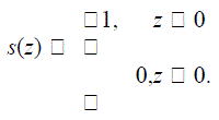
| Where’s(z) is the thresholding (step) function | ||||
 |
||||
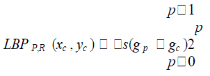
| The generic local binary pattern operator is derived from this joint distribution. As in the case of basic LBP, it is obtained by summing the threshold differences | ||||
 |
||||
| In practice, Eq. 2.10 means that the signs of the differences in a neighborhood are interpreted as a P -bit binary number, resulting in 2P distinct values for the LBP code. The local gray-scale distribution, i.e. texture, can thus be approximately described with a 2P -bin discrete distribution of LBP codes: | ||||
| In calculating the LBP P,R distribution (feature vector) for a given | ||||
| N ×M image sample (xc ∈ {0, . . . , N −1}, yc∈ {0, . . , M −1}), the central part is only considered because a sufficiently large neighborhood cannot be used on the borders. The LBP code is calculated for each pixel in the cropped portion of the image, and the distribution of the codes is used as a feature vector, denoted by S: | ||||
| S = t (LBPP,R(x, y)), x∈ {_R_, . . . , N −1−_R_}, y ∈ {_R_, . . . , M −1−_R_} (2.12) | ||||
| The original LBP is very similar to LBP8,1, with two differences. First, the neighborhood in the general definition is indexed circularly, making it easier to derive rotation invariant texture descriptors. Second, the diagonal pixels in the 3×3neighborhood are interpolated in LBP 8, 1. | ||||
| Due to its discriminative power and its computational simplicity, LBP texture operator has become a popular approach in various applications. The LBP operator detects many different texture primitives, which makes it possible to analyze images in real time settings. | ||||
EXPRESSION RECOGNITION |
||||
| Support Vector Machine is a popular technique for classification.SVM performs an implicit mapping of data in a higher dimensional feature space, where linear algebra and geometry can be used to separate data that is only separable with nonlinear rules in the input space. | ||||
| Given a training set of labeled examples |
||||
| the new test data x is classified by the following function: | ||||
| Where are Largrange multipliers of a dual optimization problem, and |
||||
| SVM finds a linear separating hyper plane with the maximal margin to separate the training data in feature space. b is the parameter of the optimal hyper plane. | ||||
| SVM allows domain-specific selection of the kernel function. Though new kernels are being proposed, the most frequently used kernel function are the linear, polynomial, and RBF kernels.SVM makes binary decisions. Here the One-Versus-Rest approach is used, which combines N-1 out of N classes into a single class and trains it against the remaining class. Multi-class classification here is accomplished by a cascade of binary classifiers together with a voting scheme. | ||||
Figures at a glance |
||||
|
||||
References |
||||
|