Keywords
|
| Hurst Edge, Compression, Segmentation |
INTRODUCTION
|
| Fractal encoding is a mathematical process used to encode bitmaps containing a real-world image as a set of mathematical data that describes the fractal properties of the image. Fractal encoding relies on the fact that all natural, and most artificial, objects contain redundant information in the form of similar, repeating patterns called fractals. |
| The encoding step in fractal image compression has high computational complexity. In this paper I briefly introduce about the Fractal image compression in chapter 1 and the various image compression techniques in chapter 2. Finally the proposed image compression techniques “Fractal Image Compression Using Hurst Edge Operator”. |
FRACTAL BASICS
|
| A fractal is a structure that is made up of similar forms and patterns that occur in many different sizes. The term fractal was first used by Benoit Mandelbrot to describe repeating patterns that he observed occurring in many different structures. These patterns appeared nearly identical in form at any size and occurred naturally in all things. Mandelbrot also discovered that these fractals could be described in mathematical terms and could be created using very small and finite algorithms and data. |
| Let's look at a real-world example. If you look at the surface of an object such as the floor currently beneath your feet, you will notice that there are many repeating patterns in its texture. The floor's surface may be wood, concrete, tile, carpet, or even dirt, but it still contains repeating patterns ranging in size from very small to very large. |
RELATED RESEARCHES
|
| A. The Hurst component and rescale analysis |
| Science is often confronted with puzzles which stay unsolved for long period s of time, one of these being the Hurst effect. The effect has been initially observed in sequences of records in time, x(t), of natural phenomena such as river discharges, which were expected to be in dependent over long periods of time. Hurst, in his analysis, first transformed the natural records in time into a new variable X(t , N), the so-called accumulated departure of the natural record in time in a given year t (t = 1, 2, ..., N), from the average , x¯(t) , over a period of N years. The transformation follows the formula |
 |
| Then, he introduced the rescaled range R/S, in which the range R(N) is def ined by and the standard deviation S(N) by |
 |
 |
| With the use of the dimensionless rescaled range, Hurst was able to compare natural phenomena of various kinds. He found, then, that the natural phenomena he studied followed the empirical law |
 |
| Where the Hurst exponent H — called K by Hurst — was more or less symmetrically distributed about a mean 0.73 with a standard deviation (SD) of about 0.09. Although this value was slightly overestimated due to the small number of available data for certain phenomena, Hurst was able to re produce the relation (2.4) by using simulations of biased random events. He derived the relation (2.5) below, which the rescaled range parameter should follow for truly unbiased events, and was able to show that his own simulations of unbiased random events obeyed it: |
 |
| This relation was also derived and discussed by Feller (1951) and later confirmed by Feder (1988) by a computer simulation of random events. Hurst’s simulations of independent random processes (1951) were done by tossing n ( =10) coins N ( = 1000) times and taking the random variable x to be the number of heads minus the number of tails. |
| Feder has, however, shown that the position in time, x(t), of a particle that walks at random with steps of unit length on a line becomes asymptotically an ordinary Brownian motion with a Gaussian distribution of step lengths for time scales much larger than the time between steps and for distances much larger than the unit step length. The variable X(t, N) of Equation (2.1) represents, in fact, the position of the particle which makes steps x(t) away from the origin. Mandelbrot later introduced a generalized form of the Brownian motion model, the fractional Brownian motion, fBm, to model the Hurst effect. In the fBm model the Hurst exponent, as shown in relation (2.3), is a real number in the range 0 < H < 1.There are three types of generalized fBm: (a) The persistent, for values of H in the range 0.5 < H < 1, (b) the anti-persistent, for 0 < H < 0.5, and (c) the case H = 0.5 which corresponds to the independent white noise processes of ordinary Brownian motion. |
| The correlation between past and future increments, C, of the accumulated Departure from the mean was estimated by Feder as |
 |
| which is notably independent of time. The correlation C takes positive values for persistent fBm, negative values for anti-persistent fBm and is zero for independent random events. Since the correlation C is in dependent of the lag time t in time series, or the number of data N when in a computer simulation of random events, the fBm predicts an infinitely long correlation in persistent and anti - persistent fBm’ s . |
| B. Fractal dimension and Hurst exponent: |
| Fractal dimension (FD) has been used to characterize data texture in a large number of fields. FD separates important classes of images and characterizes information which is not characterized by other texture features. A variety of procedures have been proposed for estimating the FD of images. These measurements are frequently referred to as dimension type- e.g., Cover Dimension (CD), Box-Counting Dimension (BCD), Hausdorff-Besicovitch Dimension (HD), Wavelet based FD, and etc. We will refer to these procedures as FD-estimators. In this section, we discuss the general concept of Rescaled Range (R/S) analysis for calculating the Hurst exponent. |
METHODOLOGY
|
| Rescaled Range analysis is a simple process that is highly data intensive. Here are the sequential steps 1. Start with the whole observed data set that covers and calculate the mean ?=(1/N)Σ ai 2. Next, sum the differences from the mean to get the cumulative total at each time point Xka from the beginning of the period up to any time: Xkm=Σ (ai – ?), k=1,2,3,…n. 3. Calculate the range R(?)= max(Xka)-min(Xka) for k=1,2,3,…n. 4. Calculate the standard deviation S, of the values, ai of the observation over the period m, for which the local mean is ?[(1/N) ? (ai – ?)2]0.5 5. Calculate R/S=R(?)/S(?). 6. For the next stage, partition the time interval in to two blocks of size N/2=? and repeat the entire procedure , steps 1-5, and determined R/S for each segment of the data set of length N/2, then take averaged value. Repeat, using successively shorter ?’s at each stage dividing the data set into non-overlapping segments and finding the mean R/S of these segments. 7. Plot the log-log plot, that is fit Linear Regression Y on X where Y=log (R/S) and X=log N. The exponent H is the slope of the regression line. |
| Example |
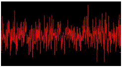
| As an example, R/S analysis has been applied to the signal shown in Figure1. The log-log plot is shown in Figure 1. The signal produces an H value of 0.3519. Because the Hurst value is different from H=0.50, we say that signal exhibits the Hurst phenomena of antipersistance. This means that if the signal had been up in the previous period, it is more likely that it will be down in the next period and vice versa. |
| B. Quincunx Neighborhood Q |
| Multifractal analysis is a new and promising approach to texture classification and image segmentation. In this method, an image I is segmented into a finite set of parts P1,P2,...,Ps which have different parameter FD such that I=?Pi, Pi?Pj=?, i?j. One of the main problems is finding the local FD. To determine such a parameter FD, it is necessary to apply a mask at each pixel. We use a special mask called Quincunx neighborhood to compute the local Hurst exponent. |
| C. Definition: A quincunx neighborhood is a set of the form:(1/2n)M-n([0,1]2) where M=[a,b]: a=[1 1]-1, b=[1,-1]-1 is the quincunx matrix and for all odd values of n. |
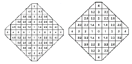
| We represent the nodes by a distance vector d whose length is equal to the number of different distances from its origin. For example, the distance vector for a Quincunx neighborhood of size 4 to one decimal place approximation is d=[1,1.4,2,2.2,2.8,3,3,2,4]. The Quincunx neighborhoods of size 5 and 4 are shown in figure 2. |
| D. Using Hurst Edge to Compress Fractal Image: |
| Over the last two decades, a wide variety of image compression techniques have been proposed [13,30,31]. The standard method uses the DCT, eliminating insignificant Fourier coefficients and storing larger ones[50]. Another method, called vector quantization, uses a building block approach, breaking up images into a small number of canonical pieces and storing only a reference to where each piece did go. Fractal image compression is a method that was introduced by M.F.Barnsley[1] and A. Jacquin[2]. Its operation is based on Iterated Functions Systems and the Collage Theorem. |
| E. Random Walks and Long Memory |
| A one dimensional random walk can be generated by starting at zero and selecting a Gaussian random number. In the next step (in this case 1), add the Gaussian random number to the previous value (0). Then select another Gaussian random number and in the next time step (2) add it to the previous position, etc... step value |
| 0 0 1 0 + R0 1 R0 + R1 2 R0 + R1 + R2 |
| Here Rn is a Gaussian random number. Random walks are sometimes referred to as Brownian motion or Gaussian noise. Figure 3.2 shows a plot of this kind of simple random walk. |
| Estimating the Hurst exponent for a data set provides a measure of whether the data is a pure random walk or has underlying trends. Another way to state this is that a random process with an underlying trend has some degree of autocorrelation When the autocorrelation has a very long (or mathematically infinite) decay this kind of Gaussian process is sometimes referred to as a long memory process. |
THE HURST EXPONENT AND FRACTIONAL BROWNIAN MOTION
|
| Brownian walks can be generated from a defined Hurst exponent. If the Hurst exponent is 0.5 < H < 1.0, the random walk will be a long memory process. Data sets like this are sometimes referred to as fractional Brownian motion (abbreviated fBm). Fractional Brownian motion can be generated by a variety of methods, including spectral synthesis using either the Fourier transform or the wavelet transform. Here the spectral density is proportional to Equation 2 (at least for the Fourier transform): |
 |
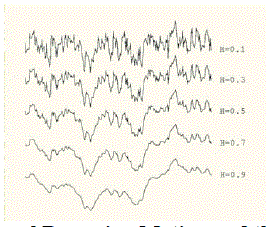
| Fractional Brownian motion is sometimes referred to as 1/f noise. Since these random walks are generated from Gaussian random variables (sets of numbers), they are also referred to as fractional Gaussian noise (or fGn). The fractal dimension provides an indication of how rough a surface is. As Equation 2 shows, the fractal dimension is directly related to the Hurst exponent for a statistically self-similar data set. A small Hurst exponent has a higher fractal dimension and a rougher surface. A larger Hurst exponent has a smaller fractional dimension and a smoother surface. This is shown in Figure 3.3. |
| A. Estimating the Hurst Exponent from the Rescaled Range |
| The Hurst exponent is estimated by calculating the average rescaled range over multiple regions of the data. In statistics, the average (mean) of a data set X is sometimes written as the expected value, E[X]. Using this notation, the expected value of R/S, calculated over a set of regions (starting with a region size of 8 or 10) converges on the Hurst exponent power function, shown in Equation 3.3. |
 |
| If the data set is a random walk, the expected value will be described by a power function with an exponent of 0.5. |
 |
| Short range dependence should have some autocorrelation (indicating some dependence between value xi and value xi+1). If there is a Hurst exponent of 0.5, it is a random walk and there is no autocorrelation and no dependence between sequential values. |
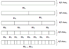
| These two values are averaged, resulting in R/S ave1. In this case the process continues by dividing each of the previous sections in half and calculating the rescaled range for each new section. The rescaled range values for each section are then averaged. At some point the subdivision stops, since the regions get too small. Usually regions will have at least 8 data points. |
| To estimate the Hurst exponent using the rescaled range algorithm, a vector of points is created, where xi is the log2 of the size of the data region used to calculate RSavei and yi is the log2 of the RSavei value. This is shown in Table 3.1. |
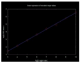
| The Hurst exponent is estimated by a linear regression line through these points. A line has the form y = a + bx, where a is the y-intercept and b is the slope of the line. A linear regression line calculated through the points in Table 3.1 results in a y-intercept of -0.7455 and a slope of 0.7270. This is shown in Figure 3.5, below. The slope is the estimate for the Hurst exponent. In this case, the Hurst exponent was calculated for a synthetic data set with a Hurst exponent of 0.72. |
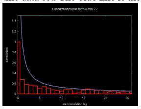
| Figure 3.6 shows an autocorrelation plot for this data set. The blue line is the approximate power curve. |
| B. Estimating the Hurst Exponent using Wavelet Spectral Density |
| The Hurst exponent for a set of data is calculated from the wavelet spectral density, which is sometimes referred to as the scalogram. The wavelet spectral density plot is generated from the wavelet power spectrum. The equation for calculating the normalized power for octave j is shown in Equation 5. |
 |
| Figure 3.7 shows the normalized power density plot for the wavelet transform of 1024 data points with a Hurst exponent of 0.72. In this case the Daubechies D4 wavelet was used. Since this wavelet octave number is the log2 of the number of wavelet coefficients, the x-axis is a log scale. |
| The Hurst exponent is calculated from the wavelet spectral density by calculating a linear regression line through a set of {xj, yj} points, where xj is the octave and yj is the log2 of the normalized power. The slope of this regression line is proportional to the estimate for the Hurst exponent. A regression plot for the Daubechies D4 power spectrum in Figure 3.7 is shown in Figure 3.8. |
| The equation for calculating the Hurst exponent from the slope of the regression line through the normalized spectral density is shown in Equation 6. |
 |
HURST BASED TEXTURE CLASSIFICATION AND SEGMENTATION
|
| Fractal based texture analysis was introduced by Pentland[3] ,where the relation between natural surface texture and fractal dimension was demonstrated. Fractal based models are useful for image segmentation, texture classification, shape-from texture and the estimation of roughness from image data. A fractal is defined as a set for which the Hausdorff-Besicovitch dimension is strictly greater than the topological dimension [5]. If TD is the topological dimension, then the fractal dimension FD can be estimated by H=TD-FD, where H is the Hurst exponent. This section, develop an efficient method for computing local Hurst exponents to measure the local roughness of an image by using the R/S technique. |
| The basic idea is to calculate the local Hurst exponents for an image. The local FD is then derived from the value of the Hurst exponent. A small value of FD represents a fine texture, while a large FD corresponds to a coarse texture. Based on this description, segment the image and find the edges with a simple thresholding method. Thresholding is the transformation of an input image I to an output binary image BI as follows: |
 |
| where T is the threshold |
| A. Hurst Edge Operator |
| Edges are often used in image analysis for finding region boundaries. The shape of edges in images depends on many parameters: the geometrical and optical properties of the object, the illumination conditions, the point spread function of the image formation process, and the noise level in the image. There are many ways to perform edge detection. However, most may be grouped into two categories, gradient and Laplacian. |
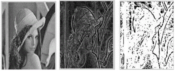
| The general idea of our method is form the slope image by the Local Hurst algorithm. Then, thresholding is applied to the slope image to form a black and white image. Since thresholding is omputationally inexpensive and fast, our method gives fast results from the slope image. Figure 3.13 shows the original image, the slope image and strong edges from the slope image. |
| First, start with an image to be compressed and then apply a two-dimensional fast wavelet algorithm with respect to an orthogonal or bi-orthogonal wavelet basis. For computational purposes, organize this process at level N as a vector C in the following manner: |
 |
| where A, H, V and D are row vectors consisting of Approximation coefficients, Horizontal detail coefficients, Vertical detail coefficients and Diagonal detail coefficients respectively, this information can be obtained by eliminating small wavelet coefficients in C . |
B. Experimental Results
|
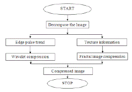
| In most cases, variations in texture are not highly visible. This suggests that to construct the image with only edge and trend information of the image. The compression ratios obtained in this method are impressive, ranging from 24 to 49 for a 512 by 512 Lena image. The image is visually similar in quality to the original image. |
| However, when the original image is subtracted from the one that has been compressed, it becomes apparent that the compression process has altered details. When the compression ratio is increased to 60:1, the appearance of artifacts throughout the image is quite apparent. |
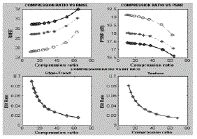
| Comparing restoration results requires a measure of image quality. Two commonly used measure Root Mean Square Error (RMSE) and Peak Signal-to-Noise Ratio (PSNR). The root mean square error between two images I(x,y) and CI(x,y) of size M*N is |
 |
 |
| where S is the maximum pixel value. Figure 3.17 shows compression ratio versus RMSE, compression ratio versus PSNR, compression ratio versus bit rate for edge trend method and compression ratio versus bit rate for texture method. |
| Figure 3.17, denote threshold values 30, 20 and 10 respectively. |
CONCLUSION AND FUTURE WORK
|
| In a progressively digital society, the role played by the compression methods is a vital one. The ever-growing need for saving more memory demands various new algorithms for highly compressed images. This paper have attempted to address issues such as a high improvement in the compression ratio while retaining the image quality, through developing image compression method Hurst Edge Operator |
SCOPE FOR FUTURE WORK
|
| The following suggestions may be considered for future work in this area. First, higher order interpolation wavelets to measure the trade-off between smoothness of large-area triangle interpolation and computational speed can be developed. |
Tables at a glance
|
 |
| Table 1 |
|
Figures at a glance
|
 |
 |
 |
 |
 |
| Figure 1 |
Figure 2 |
Figure 3 |
Figure 4 |
Figure 5 |
 |
 |
 |
 |
 |
| Figure 6 |
Figure 7 |
Figure 8 |
Figure 9 |
Figure 10 |
|
References
|
- C. M. Kung, W. S. Yang, C. C. Ku, C. Y. Wang, "Fast Fractal Image Compression Base on Block Property," icacte, pp.477-481, 2008International Conference on Advanced Computer Theory and Engineering, 2008
- RamyachitraDuraisamy, L. Valarmathi and JeyalakshmiAyyappan, Iteration Free Hybrid Fractal Wavelet Image Coder, InternationalJournal of Computational Cognition (http://www.ijcc.us), Vol. 6, No. 4, December 2008
- A. E. Jacquin. Image Coding Based on a fractal theory of Iterated Contractive Image Transformation. IEEE Transaction on Image processing, 1991,1, 1.
- M. F. Barnsley and L. Hurd. Fractal Image Compression. A. K. Peters, Wellesley, MA, 1993.
- M. F. Barnsley. Fractals Everywhere. Academic Press, 1993
- D. J. Hebert and HyungJun Kim. Image Encoding with Triangulation Wavelets. Proc. SPIE, Wavelet Applications in Signal and ImageProcessing, 2569, 1995, 381-392.
- D.J.Hebert and Ezekiel Soundararajan. Fast Fractal Image compression with Triangulation Wavelets. Proc. SPIE Conf. on WaveletApplications in Signal and Image Processing,1998
- M.F. Barnsley, and S. Demko, Iterated function systems and the global construction of fractals," Proc. Roy. Soc. Lond., vol. A399, pp. 243-275,1985.
- M.F. Barnsley, V. Ervin, D. Hardin, and J. Lancaster, \Solution of an inverse problem for fractals and other sets," Proc . Nat. Acad. Sci. USA., vol. 83, pp. 1975-1977, 1985.
- Y. Fisher, Editor, Fractal Image Compression, Theory and Application. New York: Springer-Verlag, 1995.
- Y. Fisher, T. P. Shen, and D. Rogovin, ?Comparison of fractal methodswith discrete cosine transform (DCT) and wavelets,? Proc. SPIE: NeuralStochast. Methods Image Signal Process. III, S.-S. Chen, Ed., vol. 2304, pp. 132–143, July 1994.
|