Image Segmentation Using Morphological
Operation for Automatic Region Growing

Ritu Sharma; Rajesh sharma

Image Segmentation Using Morphological Operation for Automatic Region Growing

Ritu Sharma, Rajesh sharma
CTIEMT, Jalandhar, PTU, Punjab, India

Related article at Pubmed, Scholar Google

Visit for more related articles at International Journal of Innovative Research in Computer and Communication Engineering

Abstract

Image Segmentation is a subset of an expansive field of Computer Vision which deals with the analysis of the spatial content of an image. It is used to detach regions from the rest of the image, in order to recognize them as objects. The key contributions of this paper are based on an algorithm and were executed step by step. Firstly Noisy Image was filtered with the help of various filters. Secondly Filtered Image was reconstructed with the help of Morphological Operations. Subsequently, Region Growing Technique was applied on reconstructed image and segmented image was implemented. Furthermore Segmented Image was divided into sub parts. Finally, Results are analyzed on three bases, firstly on the segmented noisy image and secondly on the filtered segmented image and finally on the sub parts of the noisy and filtered segmented image with four parameters such as PSNR (Peak Signal Noise to Ratio), MSE (Mean Square Error), Mean difference and Maximum difference.

Keywords

Image Segmentation, Gaussian Noise, Guided Filtering, Morphological Operations Automatic Region Growing

INTRODUCTION

In recent years, Automatic Image Segmentation has become a prominent intention in image analysis and computer vision. Image segmentation can be defined as the classification of all the picture elements or pixels in an image into diverse clusters that exhibit similar features [1].Image segmentation is crucial component in many signal processing technique and its applications. It aspires to congregate pixels into prominent image regions, i.e., regions equivalent to individual surfaces, items or accepted parts of objects. The outcome of image segmentation is a set of segments that cover the intact image, or a set of contours extract from the image. Digital images are prone to a multiplicity of types of noise. Noise is the consequence of errors in the image acquisition process that result in pixel values that do not imitate the accurate intensities of the authentic scene. In this paper we shall remove noise with help of guided filter. We used morphological operations to create masks along with automatic region growing technique segment the filtered image. So in this method the users don’t necessitate to opt for the seed point manually consequently there is no need of human infringement.

II. PRACTICAL METHODOLOGY

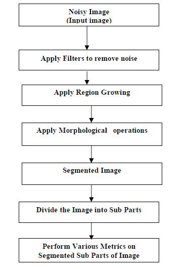
The process flow of our method is shown as figure 1. The input noisy Image is taken as an input image and then filtered with the help of filters. Gradient magnitude is to be computed after applying Morphological operations. Image segmentation is done using Region growing method. Eventually results are analyzed into 3 parts. First one represents graphical and tabular representation of Non Filtered Segmented Image with respect to four parameters, PSNR (peak signal noise to ratio), MSE (mean square error), Mean difference and Maximum difference. Second part represents graphical and tabular representation of Filtered Segmented Image with respect to four parameters PSNR (peak signal noise to ratio), MSE (mean square error), Mean difference and Maximum difference mentioned above. Third part of the results depicts the tabular form in which we represented values of Sub Parts of the Segmented Image by performing four parameters, PSNR (peak signal noise to ratio), MSE (mean square error), Mean difference and Maximum difference.

A. Image Pre-Processing

In this first step, we take an image and add noise in that image. Noise is a factor that influences image quality, which is primarily formed in the process of image acquirement and transmission. Noise appears from diverse sources in an image. The image acquisition procedure converts an optical image into an incessant electrical signal that is then sampled, is prime process by means of which noise appears in digital image. We shall add Gaussian noise.

B. Gaussian Noise

Gaussian noise is numerical noise that has a probability density function of the normal distribution. In supplementary, the values that the noise can acquire on are Gaussian-distributed. Gaussian noise is appropriately defined as the noise with a Gaussian amplitude distribution. Noise is modeled as preservative white Gaussian noise, wherever all the image pixels swerve from their original values subsequent the Gaussian curve. To facilitate is, for each image pixel with intensity value fij (1 ≤ i ≤ m, 1 ≤ j ≤ n for an m x n image), the equivalent pixel of the noisy image gij is given by, gi,j= fi,j + ni,j Where, each noise value n is drawn from a zero -mean Gaussian distribution. [4]

C. Noise Removal by Guided Filter

In second step, Gaussian noise shall be removed. This type of noise shall be removed by guided filtering. Guided filter is an unambiguous image filter, resultant from a local linear model; it generates the filtering output by taking into consideration the contented of a guidance image that can be the key in image itself or another deferent image. It has a rapid and non-approximate linear-time algorithm, whose computational complexity is autonomous of the filtering kernel size. Its output is close by a linear transform of the guidance image. The filter has the edge-preserving smoothing feature like the bilateral filter, but does not undergo from the gradient setback artifacts. Besides, the guided filter has an O (N) time (number of pixels N) correct algorithm for both gray-scale and color images. The guided filter performs well in conditions of both superiority and efficiency in a range of applications, such as noise lessening, detail smoothing/enrichment, HDR detail smoothing/ enrichment, HDR compression, image mat/feathering and haze elimination

D. Morphological Operations

Morphological Operations is a technique for the study and processing of geometrical structure, based on set hypothesis, lattice hypothesis, topology, and arbitrary functions. It is mainly recurrently applied to digital images, but it can be affianced as well on graphs, surface meshes, solids, and many advance spatial structures. It explores an image with a small form or template called a structuring element. The structuring element is situated at all potential locations in the image and it is compared with the subsequent region of pixels. Some operations test whether the element "fits" within the region, while others test whether it "hits" or intersect the region. [7] Morphological Operations includes:-

? Dilation

It is the set of all points in the image, wherever the structuring element “touches” the front. Consider each pixel in the input image, if the structuring element touches the forefront image; write a “1” at the initial point of the structuring element.

? Erosion

Erosion is the set of all points in the image, where the structuring element “fits into”. Regard as each forefront pixel in the key in image, if the structuring element fits in; write a “1” at the preliminary point of the structuring element. Pattern matching is the effortless appliance of erosion

? Opening

Opening consists of an erosion followed by a dilation and is used to exterminate all pixels in regions that are too minute to include the structuring element. Here the structuring element is frequently called a query, because it is questioning the image looking for small objects to sprain out of the image.

? Closing

Closing comprises of a dilation followed by erosion and can be used to fill in holes and small gaps.

E. Automatic Region Growing Method

The Automatic seeded region growing algorithm is one of the simplest region-based segmentation methods. It performs a segmentation on an image with examine the neighboring pixels of a set of points, acknowledged as seed points, and conclude whether the pixels could be classified to the cluster of seed point or not [8]. The algorithm procedure is as follows.

Step1. We start with a number of seed points which have been clustered into n clusters, called C1, C2… Cn. And the position of initial seed points is set as p1, p2… p3.

Step2. To compute the difference of pixel value of the initial seed point pi and its neighboring points, if the difference is smaller than the threshold (criterion) we define, the neighboring point could be classified into Ci, where i = 1, 2, …,n.

Step3. Recomputed the boundary of Ci and set those boundary points as new seed points pi (s). In addition, the mean pixel values of Ci have to be recomputed correspondingly.

Step4. Repeat Step2 and 3 until all pixels in image have been allocated to a suitable cluster.

III. IMPLEMENTATION

Implementation has been done in two parts:-

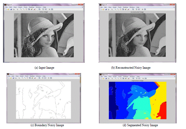
a) Segmentation without removing noise i.e. Non-Filtered image.

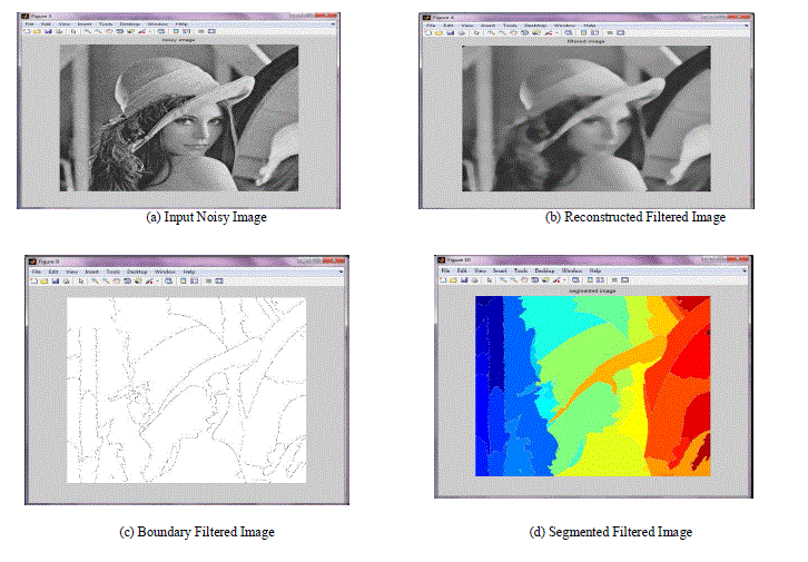
b) Segmentation by removing noise i.e. with Filtered image.

A. Segmentation without removing noise i.e. Non-Filtered image

B. Segmentation without removing noise i.e. Filtered image

IV. RESULTS

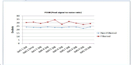
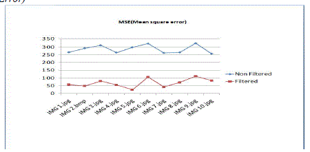
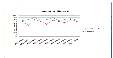
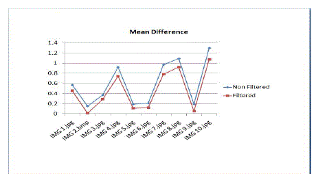
This section represents graphical representation with respect to four parameters psnr (peak signal noise to ratio), MSE (mean square error), mean difference and maximum difference among non filtered and filtered segmented image.

A.PSNR (Peak Signal Noise to Ratio)

B. MSE (Mean Square Error)

C. Maximum Difference

D. Mean Difference

V. CONCLUSION

This is region growing segmentation method for segmenting noisy and filtered images.we proposed a new, robust, fast and fully automatic algorithm. The algorithm needs no prior information or training process.we successfully find the seed points and the segmentation results obtained are very much accurate. By analysing on four different parameters,we did comparision between non filtered and filtered image. This method gives better results compared to other methods.

Figures at a glance


Figure 1	Figure 2	Figure 3	Figure 4

Figure 5	Figure 6	Figure 7

References

Luis Garcia Ugarriza, Eli Saber, Senior Member, IEEE, Sreenath Rao Vantaram, “Automatic Image Segmentation by Dynamic Region Growthand Multiresolution Merging”, IEEE TRANSACTIONS ON IMAGE PROCESSING, VOL. 18, NO. 10, OCTOBER 2009.

Ashraf A. Aly, Safaai Bin Deris, NazarZaki, “Research review for digital image segmentation techniques”, International Journal of ComputerScience & Information Technology (IJCSIT) Vol 3, No 5, Oct 2011

Chi Chang-yanab, Zhang Ji-xiana, Liu Zheng-juna”Study on methods of noise reduction in a stripped image”, The International Archives of thePhotogrammetry, Remote Sensing and Spatial Information Sciences. Vol. XXXVII Part B6b. Beijing 2008.

GnanambalIlango and R. Marudhachalam, “New hybrid filtering techniques for removal of Gaussian noise from medical images”, ARPN Journalof Engineering and Applied Sciences, VOL. 6, NO. 2, FEBRUARY 2011.

Sonali R. Mahakale&Nileshsingh V. Thakur, “A comparative study of image filtering on various noisy pixels”, International Journal of ImageProcessing and Vision Sciences ISSN (Print): 2278 – 1110, Volume-1, Issue-2, 2012.

Aditya Goyal, AkhileshBijalwan, “Image Enhancement using Guided Image Filter Technique ”,International Journal of Engineering andAdvanced Technology (IJEAT),ISSN: 2249 – 8958, Volume-1, Issue-5, June 2012 .

http://www.cs.auckland.ac.nz

R. Adams, and L. Bischof, “Seeded region growing,” IEEE Trans. Pattern Anal Machine Intel., vol. 16, no. 6, pp. 641-647, June, 1994.

http://disp.ee.ntu.edu.tw.

P.RajaSekharReddy,N.NagaLakshmi,ThanduAshalatha,“Image Segmentation Using A Region Growing Method”, Ijess, Volume2, Issue7,July-2012.

D. Muhammad Noorul Mubarak, M. Mohamed Sathik, S.ZulaikhaBeevi and K.Revathy, “A hybrid region growing algorithm for medical imagesegmentation”, International Journal of Computer Science & Information Technology (IJCSIT) Vol. 4, No 3, June 2012.

B. Senthilkumar1 and G. Umamaheswari, “A new region growing segmentation algorithm for the detection of breast cancer”, InternationalJournal of Computer Science and Communication, Vol. 3, No. 1, January-June 2012.

Peter Yu, A. K. Qin, Member, IEEE, and David A. Clausi, Senior Member, IEEE,“UnsupervisedPolarimetric SAR Image Segmentation andClassification Using Region Growing With Edge Penalty”, IEEE Transactions on Geosciences and Remote Sensing, Vol. 50, No. 4, April 2012.

Sonali r. Mahakale&Nileshsingh v. Thakur, “A comparative study of image filtering on various noisy pixels”, International Journal of ImageProcessing and Vision Sciences ISSN (Print): 2278 – 1110, Volume-1, Issue-2, 2012.

Rashmi Saini, MaitreyeeDutta and Robin Kumar, “A comparative study of several image segmentation techniques”, Journal of Information andOperations Management, ISSN: 0976–7754 & E-ISSN: 0976–7762, Vol. 3, Issue 1, 2012.

Mukesh Kumar, Kamal K.Mehta, “A Texture based Tumor detection and automatic Segmentation using Seeded Region Growing Method”,IJCTA, Vol 2 (4), 855-859, July-August 2011.