Market analysis is an important component of analytical system in retail companies to determine the sales for different segments of customers to improve customer satisfaction and to increase profit of the company which has different channels and regions. These issues for a leading shopping mall is addressed using frequent item set mining and decision tree technique. The frequent item sets are mined from the market basket database using the efficient Apriori algorithm and hence the association rules are generated. The decision tree can be constructed using ID3 and C4.5 algorithm.
Keywords |
| Association Rules, Frequent Item sets, Apriori, Decision tree, Market Basket Analysis |
INTRODUCTION |
| One of the challenges for companies that have invested heavily in customer data collection is how to extract
important information from their vast customer databases and product feature databases, in order to gain competitive
advantage. Several aspects of market basket analysis have been studied in academic literature, such as using customer
interest profile and interests on particular products for one-to-one marketing, purchasing patterns in a multi-store
environment to improve the sales [1]. Market basket analysis has been intensively used in many companies as a means
to discover product associations and base a retailer’s promotion strategy on them. Informed decision can be made easily
about product placement, pricing, promotion, profitability and also finds out, if there are any successful products that
have no significant related elements [2]. Similar products can be found so those can be placed near each other or it can
be cross-sold. A retailer must know the needs of customers and adapt to them. Market basket analysis is one possible
way to find out which items can be put together. Market basket analysis gives retailer good information about related
sales on group of goods basis and also it is important that the retailer could know in which channel and in which region
the products can be sold more and which session (i.e) morning or evening [3]. |
| Market basket analysis is one of the data mining methods focusing on discovering purchasing patterns by
extracting associations or co-occurrences from a store’s transactional data. Market basket analysis determines the
products which are bought together and to reorganize the supermarket layout and also to design promotional campaigns
such that products’ purchase can be improved [11]. Association rules are derived from the frequent item sets using
support and confidence as threshold levels [4]. The sets of items which have minimum support are known as Frequent
Item set [2]. The support count of an item set is defined as the proportion of transactions in the data set which contain
the item set. Confidence is defined as the measure of certainty or trustworthiness associated with each discovered
pattern. Association rules derived depends on confidence [5]. |
II. RELATED WORK |
| A number of approaches have been proposed to implement data mining techniques to perform market analysis.
Loraine et al. in their work proposed a market basket analysis using frequent item set mining. They compared
Apriori with K-Apriori algorithm to find the frequent items [1]. Vishal et al. implemented data mining in online shopping system using Tanagra tool. They made decision about the placement of product, pricing and promotion
[2]. |
| Sudha and Chris et al. proposed the impact of customers perception and crm on indian retailing in the changing
business scenario using data mining techniques[3][4]. Comparing to the works discussed above, our work is different
by using apriori and decision tree to perform market basket analysis. |
III. SYSTEM ARCHITECTURE |
A. Customer data set: |
| The Wholesale customer data provided by the UCI Machine Learning Repository is used for analysis of this
work [7]. The dataset has 8 continuous and 1 numeric input attributes namely channel, region, fresh, milk, grocery,
frozen, detergents, delicatessen and session. |
| It also has the predicted attribute i.e) the class label. Here the channel1 represents horeca
(hotel/restaurant/café), channel2 represents retail shops. Region1 represents Lisbon, region2 represents Oporto,
region3 represents the others. The description of the dataset is tabulated in Table 1. |
B. Association Rules: |
| Association rules are of the form if X then Y. Frequent patterns is patterns (such as item sets, subsequences, or
substructures) that appear in a data set frequently [6]. Frequent pattern mining searches for recurring relationships in a
given data set. Association rules are not always useful, even if they have high support, confidence and lift > 1.
Association rules can also be improved by combining purchase items. Items often fall into natural hierarchies. In This Section, frequent item set can be generated using apriori algorithm and associate outliers also be generated according to
the given support count and confidence level. |
C. Decision tree: |
| Decision tree induction is the learning of decision trees from class-labeled training tuples. Decision tree
algorithms, such as ID3, C4.5, and CART, were originally intended for classification. Decision tree induction
constructs a flow chart like structure where each internal (non leaf) node denotes a test on an attribute, each branch
corresponds to an outcome of the test, and each external (leaf) node denotes a class prediction. The topmost node in a
tree is the root node. The construction of decision tree classifiers does not require any domain knowledge or parameter
setting, and therefore is appropriate for exploratory knowledge discovery [13]. |
| Decision trees can handle high dimensional data. Their representation of acquired knowledge in tree form is
intuitive and generally easy to assimilate by humans. The learning and classification steps of decision tree induction are
simple and fast. In general, decision tree classifiers have good accuracy. Decision trees are the basis of several
commercial rule induction systems. At each node, the algorithm chooses the “best” attribute to partition the data into
individual classes [13]. |
ID3: |
| ID3 uses information gain as its attribute selection measure. The expected information needed to classify a
tuple in D is given by |
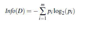 |
| where pi is the probability that an arbitrary tuple in D belongs to class Ci and is estimated by jCi,Dj/jDj [4]. A log
function to the base 2 is used, because the information is encoded in bits. Info (D) is just the average amount of
information needed to identify the class label of a tuple in D[8]. |
| InfoA(D) is the expected information required to classify a tuple from D based on the partitioning by A. The smaller
the expected information (still) required, the greater the purity of the partitions. This can be measured by |
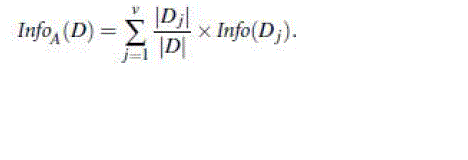 |
| The term Dj acts as the weight of the jth partition. Information gain is defined as the difference between the original
information requirement (i.e., based on just the proportion of classes) and the new requirement (i.e., obtained after
partitioning on A). That is, |
 |
C4.5: |
| C4.5 is an algorithm used to generate a decision tree developed by Ross Quinlan. The decision trees
generated by C4.5 can be used for classification, and for this reason, it is often referred to as a statistical classifier.
C4.5, a successor of ID3, uses an extension to information gain known as gain ratio, which attempts to overcome this
bias. C4.5 builds decision trees from a set of training data in the same way as ID3, using the concept of information
entropy. The training data is a set S=s1, s2... of already classified samples |
| Each sample si consists of a p-dimensional vector (x1,i,x2,i,...,xp,i), where the xj represent attributes or
features of the sample, as well as the class in which si falls. At each node of the tree, C4.5 chooses the attribute of the
data that most effectively splits its set of samples into subsets enriched in one class or the other. |
| It applies a kind of normalization to information gain using a “split information” value defined analogously
with Info (D) as |
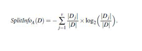 |
| This value represents the potential information generated by splitting the training data set, D, into v partitions,
corresponding to the v outcomes of a test on attribute A [9]. |
| Note that, for each outcome, it considers the number of tuples having that outcome with respect to the total
number of tuples in D [5]. It differs from information gain, which measures the information with respect to
classification that is acquired based on the same partitioning. The gain ratio is defined as |
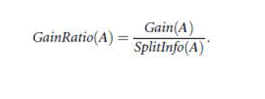 |
| The attribute with the maximum gain ratio is selected as the splitting attribute[15]. |
| Here also the error rate and the confusion matrix of ID3 can be found and for the given dataset the decision tree
can be generated by |
| • Channel < 1.5000 |
| • Region < 2.5000 then session = morning(54.02 % of 87 examples) |
| • Region >= 2.5000 then session = evening(58.77 % of 211 examples) |
| • Channel >= 1.5000 |
| • Region < 1.5000 then session = evening (72.22 % of 18 examples) |
| • Region >= 1.5000 then session = morning(56.45% of 124 examples) |
| This is the simple decision tree for three attributes channel, region and session. |
| If we construct the decision tree for the whole dataset it becomes very efficient with the accuracy of 72.22%
maximum [10]. |
IV. SIMULATION RESULTS |
| The whole dataset was given to the data mining tool like Tanagra. Then frequent item set is found using apriori
algorithm in the association technique [12]. This paper is mainly focused to find out whether the products can be sold
more at morning session or evening session. For this, it uses two decision tree algorithms called ID3 and C4.5. Using
ID3 the dataset parameters can be splitted and also found the error rate with confusion matrix [13]. Using C4.5
algorithm, the decision tree can be constructed for the given confidence level and minimum size of leaves [6]. |
| The statistical analysis of the whole dataset is given in Table 3. It gives the mean and accuracy of the product sold in
two sessions |
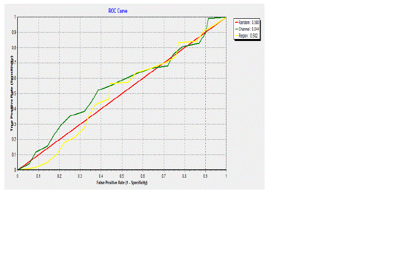
| A receiver operating characteristic (ROC) curve is a graphical plot that illustrates the performance of a binary
classifier system as its discrimination threshold is varied. The curve is created by plotting the true positive rate against
the false positive rate at various threshold settings. |
| The ROC curve of our work is shown in Fig. 2. Here the positive value should be taken as morning and the result
becomes nearly true positive is little bit higher than the false positive [14]. This diagram illustrates at what channel and
region our products sends more in the morning and whether it gets true positive or not. |
V. CONCLUSION |
| In this paper, a framework for Decision tree and frequent item set is developed for the analysis of wholesale
data. The wholesale customer dataset is taken and analyzed to know the session at which the product can be sold more
using decision tree algorithm like ID3 and C4.5. The data in the dataset is preprocessed to make it suitable for
classification. The preprocessed data is used for classification and we obtained high classification accuracy. |
Tables at a glance |
|
|
| |
Figures at a glance |
 |
 |
| Figure 1 |
Figure 2 |
|
| |
References |
- Loraine Charlet Annie M.C.1 and Ashok Kumar D, âÃâ¬ÃÅMarket Basket Analysis for a Supermarket based on Frequent Itemset MiningâÃâ¬ÃÂ, IJCSIInternational Journal of Computer Science Issues, Vol. 9, No. 3, pp.257-264, 2012.
- Vishal jain, Gagandeepsinghnarula&Mayanksingh, âÃâ¬ÃÅImplementation of data mining in online shopping system using Tanagra toolâÃâ¬ÃÂ,International journal of computer science And engineering Vol. 2, No. 1, 2013.
- Sudha vemaraju, âÃâ¬ÃÅChanging waves in indian retailing: Impact of customers perception and crm on indian retailing in the changing businessscenarioâÃâ¬ÃÂ, International Journal of Multidisciplinary Research , Vol.1, No.8, 2011.
- Chris Rygielski, Jyun-Cheng Wang b, David C. Yen, âÃâ¬ÃÅData mining techniques for customer relationship managementâÃâ¬ÃÂ, Technology in Society,2002.
- P Salman Raju, Dr V Rama Bai, G Krishna Chaitanya, âÃâ¬ÃÅData mining: Techniques for Enhancing Customer Relationship Management inBanking and Retail IndustriesâÃâ¬ÃÂ, International Journal of Innovative Research in Computer and Communication Engineering Vol. 2, No.1, 2014.
- Bharati M Ramager, âÃâ¬ÃÅData Mining techniques and ApplicationsâÃâ¬ÃÂ, International Journal of Computer Science and Engineering, Vol. 8, No.12,2009.
- P. Nancy, and Dr. R. GeethaRamani, âÃâ¬ÃÅA Comparison on Data Mining Algorithms in Classification of Social Network DataâÃâ¬ÃÂ,InternationalJournal of Computer Applications, Vol.32, No.8, 2011.
- Sheikh, L Tanveer B. and Hamdani, "Interesting Measures for Mining Association Rules", IEEE Conference-INMIC , 2004.
- Sonali Agarwal, Neera Singh, Dr. G.N. Pandey, âÃâ¬ÃÅImplementation of Data Mining and Data Warehouse in E-GovernanceâÃâ¬ÃÂ, International Journalof Computer Applications, Vol.9, No.4, 2010.
- Chen, Y.-L., Tang, K., Shen, R.-J., Hu, Y.-H.:âÃâ¬ÃÂMarket basket analysis in a multiple store environmentâÃâ¬ÃÂ, Journal of Decision Support Systems,2004.
- Berry, M.J.A., Linoff, G.S.: âÃâ¬ÃÅData Mining Techniques: for Marketing, Sales and Customer Relationship ManagementâÃâ¬Ã (second edition),Hungry Minds Inc., 2004.
- C. Rygielski, J. C. Wang, and D. C. Yeh, "Data mining techniques for customer relationship management," Technology in Society, vol. 24,2002.
- J. Han and M. Kamber, âÃâ¬ÃÅData Mining : Concepts and TechniquesâÃâ¬ÃÂ, San Francisco: Morgan Kaufmann Publisher, 2006.
- H. Jantan, A. R. Hamdan, Z. A. Othman, and M. Puteh, "Applying Data Mining Classification Techniques for Employee's PerformancePrediction," 5th International Conference in Knowledge Management, 2010.
- Rastogi, R..andkyuseok Shim, âÃâ¬ÃÅMining optimised association rules with Categorical and numerical attributesâÃâ¬ÃÂ, IEEE transactions onKnowledge and Data Engineering, vol.14, No.2, pp.425-439, 2002.
|