Keywords
|
| Data compression, Rice algorithm, Curve fitting, Verilog. |
INTRODUCTION
|
| The Lossless Data Compression technique preserves the source data accuracy by removing redundancy from the application source data, which allows the exact original data to be reconstructed from the compressed data. In the decompression processes the original source data is reconstructed from the compressed data by restoring the removed redundancy [5]. The reconstructed data is an exact replica of the original source data. Lossless compression is used in cases where it is important that the original and the decompressed data be identical, or where deviations from the original data could be deleterious [7]. Lossless data compression has been suggested for many space science exploration mission applications either to increase the science return or to reduce the requirement for on-board memory, station contact time, and data archival volume. |
| Lossy compression reduces bits by identifying unnecessary information and removing it. Lossy methods are most often used for compressing sound, images or videos. Lossless compression schemes are reversible so that the original data can be reconstructed, while lossy schemes accept some loss of data in order to achieve higher compression [5]. |
RICE ALGORITHM
|
| In Rice algorithm, variable-length coding compression method is used [1]. Variable-length coding, is the compression method in which shorter code words are assigned to data that are expected to occur with higher frequency [6]. The main advantage of Rice algorithm is that it can adapt to low entropy to high entropy sources. |
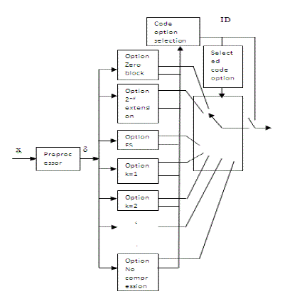
| In Fig. 1 a block diagram of the Rice algorithm is shown. |
| It consists of a mainly two parts, a pre-processor and an adaptive entropy coder. The function of the pre-processor is to decorrelate data samples and then maps them into symbols suitable for the adaptive entropy coder [1]. |
| A. Compression options in Adaptive Entropy coder |
| The different compression options available are [1], [2]: |
| • Fundamental sequence encoding |
| • The split-sample options |
| • Low entropy options |
| • No compression option |
| The option that gives maximum compression for a given set of data is selected. |
| B. The pre-processor |
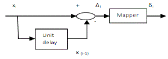
| 1) Predictor: One of the simplest predictive coders is a linear first-order unit-delay predictor shown in Fig.2. |
| In Fig. 2 output, Δi, will be the difference between the input data symbol and the preceding data symbol, and is called as prediction error. δi is called the prediction error mapping function [1]. |
| 2) The mapper: Based on the predicted valueïÿýïÿý ïÿýïÿý , the prediction error mapper converts each prediction error value, Δi, to an n-bit nonnegative integer, δi, suitable for processing by the entropy coder [6]. |
| Table I illustrates the operation of the prediction error mapper after a unit-delay predictor is applied to 8-bit data samples of values from 0 to 255[1], [ 2]. |
| The prediction error mapping function: |
 (1) (1) |
 (2) (2) |
MODIFIED RICE ALGORITHM USING CURVE FITTING
|
| Curve fitting is the process of a curve or a mathematical function that best suits to a set of data points. An equation is produced by curve fitting that can be used to find points anywhere along the curve [3], [8]. It can involve interpolation, where a smooth function that fits exactly to the data is required. When the fitted curve is used beyond the range of data set, it is referred to as extrapolation. Thus prediction of next data value (ïÿýïÿý ïÿýïÿý ) is possible with this method [11]. For a set of inputs a unique function is assigned, this function is updated for different set of inputs [4]. |
| A. Polynomial curve fitting in modified rice algorithm |
| The general form for a polynomial of order j is given by : |
 (3) (3) |
| using least square curve method here, so that a curve that gives minimum error between the data (y) and the function f(x) is obtained finally. |
| The general expression for any error using the least squares approach is: |
 (4) (4) |
| Substitute the form of eq. (3) into general least square error eq. (4) |
 (5) (5) |
| where n-number of data points, i-current data point,j-order of the polynomial. |
| The best suited curve will give minimum error between line and data points [10]. So the objective is to minimize the eq. (5) and also find the corresponding values of the coefficients ak, a0. To minimize eq. (5), take the derivative of Error with respect to each coefficient a0 , ak where k=1, 2….j, set each value to zero. |
 (6) (6) |
| Representing the equation using a matrix form as follows |
| where i =1…………..n |
| To know the value of a0, ak, solve eq. (7).For that take |
 () () |
| The following solution method can be used: |
 (7) (7) |
| Therefore |
 (8) (8) |
| Using equation (8) the values of coefficients a0,ak are found out and finally a polynomial equation that fits for the data points is obtained[4].The coefficient values are then quantized, these values are then implemented in the function which is used to predict the next set of values. The quantized function coefficients along with the δ values and the ID that represents the compression option used are transmitted to the receiver[1]. As a result at the receiver the data can be reconstructed without any error that means these results in lossless compression. |
| B. Special case of modified rice algorithm |
| In special cases a method is implemented using modified rice algorithm to obtain higher compression. The special case is applicable when the input signal for compression and the signal obtained by curve fitting overlap at the initial stage. The existing rice algorithm finds the corresponding delta (δ) values and applies the compression option to all δ values. The modified rice algorithm excludes the initial δ=0 values and then applies the compression option. The special case is explained with an example. |
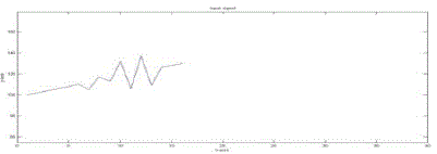
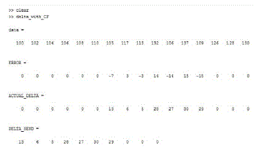
| In Fig. 3 input signal for special case is shown |
| Fig. 4 shows the delta values obtained using rice algorithm for the input signal shown in Fig. 3 |
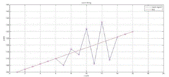
| Fig. 5 shows the graph of input signal and the function which is obtained through curve fitting in modified rice algorithm |
| In Fig. 6 actual delta values and delta values obtained under special case is shown.Delta values obtained through special case has less number of values than actual delta values |
| To understand the use of modified rice algorithm based on curve fitting represented in Fig. 5 and Fig. 6 consider the above example. If the values of δ contains a block of zeros followed by other numbers, that is, if the δ values are 0,0,0,0,0,0,13,6,5,28,27,30,29,0,0,0 |
| then, less number of bits are required to transmit this data when modified rice algorithm is used. This is because the initial 6 zeros are not taken for further proceedings (i.e. compression options are not applied on these initial zero values). So the best compression option can be selected taking only the δ values starting from δ =13 to δ =0.Thus the transmitted data will consist of fewer bits. As the number of samples in a block of data is constant (in the example, number of samples in block is 16) at the receiver the data is reconstructed back by filling the locations not specified with zero. |
SIMULATION RESULTS AND COMPARATIVE STUDY
|
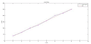
| In Fig. 7 graph of 8 input samples and curve fitting function is shown |
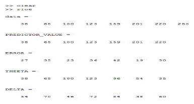
| In Fig. 8 output obtained during mapping rice algorithm is shown |
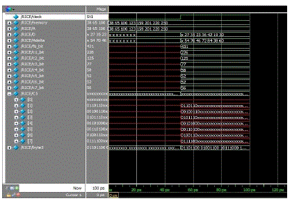
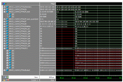
| Fig. 9 shows the output waveform using rice algorithm, which is obtained as the simulation result in ModelSim using Verilog HDL.C5 and byte5 represent compressed data using 5th split sample option |
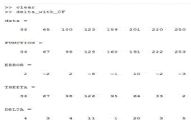
| Fig. 10 shows the values obtained during mapping using modified rice algorithm. FUNCTION values are obtained through curve fitting |
| In Fig. 11 output waveform of modified rice algorithm showing compressed data is shown,which is obtained as the simulation result in ModelSim using Verilog HDL. |
| For simulation using ModelSim the input data is read from file to variable A. The function parameters (f_mat) are calculated and quantized (f_mat_quantized). The function (f) values at each point are calculated using these quantized values. Further δ (Adelta) values are determined. Adelta is compressed using all possible compression options and the compressed data with least number of bits is chosen for transmission. Here 2nd split sample option (C2) is chosen as the number of bits (c2_bit) is minimum when compared with other options used. Compressed data bits in C2 is converted to bytes and stored in byte2. |
| For the above example the number of bits in compressed data is 52 (Fig. 9 c5_bit) when rice algorithm is used. Whereas the number of bits in compressed data is 34 (Fig: 11 c2_bit) when modified rice algorithm is used. Thus the number of bits of compressed data reduces when modified rice algorithm is used. |
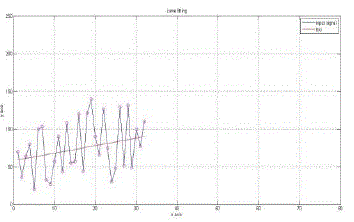
| Fig. 12 represents a highly varying input and curve fitted signal |
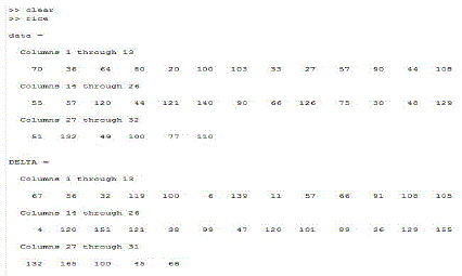
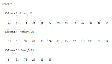
| Fig. 13 shows the mapped delta values for the input in Fig. 12 using rice algorithm |
| Fig. 14 shows mapped delta values for input in Fig. 12 obtained using modified rice algorithm |
| In the above figures the variables named as delta, error, theta etc. are found out by subtracting the predicted value from the data value and using eq. (1) & (2), in the case of Rice algorithm. Here even if there are n inputs, only (n-1) outputs are present at the output because of the unit delay predictor. |
| In the case of curve fitting a particular function is assigned to the data set, with which next values can be predicted and then the error values can be calculated by subtracting the predicted value from the data value and delta and theta values are obtained using the eq. (2) & (3).Here if there are n inputs present, at the output also there will be n values |
| A. Comparison between rice algorithm and modified rice algorithm based on curve fitting |
| • In rice algorithm, we predict that the next data will be similar to that of the current data. |
| Whereas in modified rice algorithm based on curve fitting, a function is developed for the given set of inputs and so data can be predicted according to the function. This results in smaller δ values. When these δ values are taken for compression, the final compressed data consist of fewer bits as compared to existing rice algorithm. Thus by using curve fitting the data bits transmitted reduces drastically. This results in higher compression ratio |
| • In rice algorithm, after compression while sending the data to the receiver, a reference value which is the first input data, (n-1) values of δ and the ID corresponding to the compression option used are transmitted. |
| Whereas in modified rice algorithm the function coefficients, n values of δ and the ID corresponding to the compression option are transmitted to the receiver. |
| • Modified rice algorithm employs lossless compression. Thus the exact signal can be reconstructed at the receiver without any losses. |
| • Higher compression is possible when special case of modified algorithm is applicable. |
CONCLUSION
|
| In this paper comparison between rice algorithm and modified rice algorithm based on curve fitting was done. To evaluate the performance of modified rice algorithm different real world signals are given and the corresponding outputs are noted, which is then compared with the output of rice algorithm for the same set of inputs. In modified rice algorithm with curve fitting, a function is generated based on the input data set, with which upcoming values are predicted. Rice algorithm is used only for those sets of data where redundancy exists. But with modified rice algorithm, in which curve fitting was implemented can be used for any real time signals which varies in a particular manner. Thus later method finds numerous applications in most of the industries where large variation of data may occur, for eg.process control industries. The simulation result shows that the data is compressed more with modified rice algorithm when a real world signal is used. With lossless compression using modified rice algorithm with curve fitting technique, it is possible to reconstruct the original signal. |
Tables at a glance
|
 |
| Table 1 |
|
Figures at a glance
|
 |
 |
 |
 |
 |
| Figure 1 |
Figure 2 |
Figure 3 |
Figure 4 |
Figure 5 |
 |
 |
 |
 |
 |
| Figure 6 |
Figure 7 |
Figure 8 |
Figure 9 |
Figure 10 |
 |
 |
 |
 |
| Figure 11 |
Figure 12 |
Figure 13 |
Figure 14 |
|
References
|
- CCSDS (Consultative committee for space data systems), GREEN BOOK ISSUE-2, December 2006
- CCSDS, BLUE BOOK ISSUE-2, May 2012
- Medioni, Gerard, and Yoshio Yasumoto. "Corner detection and curve representation using cubic< i> B</i>-splines." Computer Vision, Graphics,and Image Processing 39.3 (1987): 267-278.
- Richardson, Mark H., and David L. Formenti. "Global curve fitting of frequency response measurements using the rational fract ion polynomialmethod."International Modal Analysis Conference. 1985.
- S. Khalid, Introduction to Data Compression, 2nd ed. San Mateo,CA: Morgan Kaufmann, 2000.
- R. F. Rice and J. R. Plaunt, “Adaptive variable length coding for efficient compression of spacecraft television data,” IEEE Trans. Commun. Techno.Vol. COM-19, part I, pp. 889-897, Dec. 1971.
- T. A. Welch, “A technique for high-performance data compression,” IEEE Trans. Comput. vol. 17, no. 6 pp. 8-19, June 1984.
- Saux, E., and M. Daniel. "Data reduction of polygonal curves using B-splines."Computer-aided design 31.8 (1999): 507-515.
- Leung, Maylor K., and Yee-Hong Yang. "Dynamic two-strip algorithm in curve fitting." Pattern Recognition 23.1 (1990): 69-79.
- Ichida, Kozo, Takeshi Kiyono, and Fujiichi Yoshimoto. "Curve fitting by a one-pass method with a piecewise cubic polynomial." ACM Transactionson Mathematical Software (TOMS) 3.2 (1977): 164-174.
- Vickers, Thomas J., Ronald E. Wambles, and Charles K. Mann. "Curve fitting and linearity: data processing in Raman spectroscopy." AppliedSpectroscopy55.4 (2001): 389-393.
|