Keywords
|
| Fault classification, differential protection, Back propagation neural network, radial basis neural network. |
I. INTRODUCTION
|
| The demand for electricity is increasing. It is very important to supply quality power continuously. It is the task of power-suppliers to maintain supply even when disturbances occur. Power system faults not only cause discontinuity in supply but also cause equipment damage. For protection a protective relay is used which clearly distinguish between faulty and normal signal. |
| Modern power transformer is one of the most vital device and its protection is crucial. One of the most effective transformer protection is differential protection. This protection is focused on discriminating faulty signals from normal signals. If for normal signal false tripping occurs then it causes discontinuity in supply. So false tripping cases should be avoided. That is relay performance should be improved. Our present work focuses on improved fault classification to avoid false tripping. |
II. LITERATURE REVIEW
|
| Power transformer is one of the important equipment in power system.One of the effective method for protection of transformers is differential protection. Basic theory of differential protection of transformers is discussed in [1]. The main difficulty for conventional differential protection is that they induce differential relay to release a false trip signal without the existing of any fault. This condition mainly occurs due to magnetizing inrush current during intial energization condition [1,5]. Therefore, to clearly classify inrush and faulty signal differential relay algorithm has to be modified.In [1-6] different differential protection algorithms are discussed. In [5] how inrush is caused, factors affecting inrush current, problems caused by inrush current are discussed. |
| In [1] digital differential relay algorithm is used which works on harmonic restraint principle. In this method there is both amplitude comparision and harmonic comparision. This uses simulation technique in MATLAB Simulink environment. This differential relay algorithm is used in this paper. |
| Now to future improve the fault classification we use AI. Different types of ANN are used for distinguishing faulty signal and normal signal. In [8-13] include application of neural networks in power system. In [10,11] explain how ANN can be used as a classifier which uses back propagation method. In [8] ANN is used to discriminate between magnetizing inrush current and internal fault current and also used to determine the type of fault that occur in a power transformer. |
| In [14,15] radial basis neural network is used as a fault classifier. This RBNN has less exection time and fastest creation of network objects. |
| In the light of above literature review we will model the differential realy. Then we will select different conditions. For this different conditions datas are generated.Using this data ANN is trained. And then ANN based relay is tested. |
| In this paper section IV describes a brief architecture of ANN employed. In section V we describe the work methodology. This is the major section in which we describe the work flow. In this section we well describe about the differential relay modeling, data generation for different conditions selected, training of ANN and finally testing and results. In section VI we conclude with a summary of major contributions from this work and observations |
III. NEURAL NETWORK ARCHITECTURE
|
| Here we use two types of neural network. Firstly we will discuss about the architecture of BPNN. Then we will discuss about the architecture of RBNN. |
III.1 BACK PROPAGATION NEURAL NETWORK
|
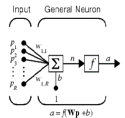
| The BPNN is a common model in neural network application. This network consists of an input layer representing the input data to the network, some hidden layers and an output layer representing the response of the network. Each layer consists of a certain number of neurons; each neuron is connected to other neurons of the previous layer through weights w and biases b as shown in Fig 1.f is any differential transfer function, most frequently used functions are sigmoid and tan sigmoid functions. |
| The learning process of BPNN is a error correction learning methods The process includes forward propagation and back propagation. In forward propagation process, the input signals pass through the input and propagate to the hidden layer and output layer. If the expected results are not obtained at the output layer, then back propagation begins. The error signals are transmitted along the coming paths for modifying the connecting weight coefficients between nodes to make the output error smallest. The above network is created by using neural network tool box in MATLAB. |
III.2 RADIAL BASIS NEURAL NETWORK
|
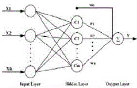
| RBNN is based on supervised learning. The network consists of input layer, hidden layer and output layer. The input layer feeds the input data, to the hidden layer. In the present work, the input data is signal that is fed to the differential relay which will be discussed in next section. The hidden layer works by neurons loaded with radial basis activation function. The output layer is powered with neurons of linear activation function. The architecture of RBNN shown in Fig 2 |
| The network inputs k input nodes and m hidden neurons. For a ïÿý dimension data ïÿý′ the network computes the scalar value ïÿý. |
 |
| where is the weight bias, is the weight parameter is the Radial basis function. The radial basis function for input is . The plot of the radial basis function is Gaussian double sided bell curve. In the present work the network iteratively creates radial basis network one neuron at a time. Neurons are added to the network until the sum-squared error falls beneath an error goal or a maximum number of neurons have been reached. The above network is created by using neural network tool box in MATLAB. |
IV. WORK METHODOLOGY
|
| Work methodology include the power system model, differential relay modeling, data generation for ANN, training of ANN and finally testing of ANN. These steps will be discussed in detail in the following sections. |
IV.1 POWER SYSTEM MODELLING
|
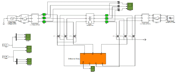
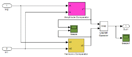
| The power system used as work background is shown in simulink model [1] in Fig 3.In this model a three phase,500kVA, 50Hz, (11/33)kV, Y/Y power transformer is used in this system. Three phase source of 11kV, 50Hz is used in the primary side of the transformer. Three phase load of 45kW is used in the secondary side of the transformer. CTs are connected on both sides of the transformer and output of these CTs are connected to the differential relay. Differential relay is shown as a subsystem in the model. Differential relay consists of amplitude comparator and harmonic comparator and this is shown in simulink model [1] is shown in Fig 4. Amplitude comparator and harmonic comparator are shown as subsystems. Modelling of amplitude and harmonic comparator is shown in [1]. |
| IV.2 FAULT CLASSIFICATION SCHEME |
| Step1. Model the differential relay. |
| Step 2. Generate the training data for faulty and normal cases. |
| Step 3. Train the network with the data generated. |
| Step 4. Test the model and validate the scheme. |
| The above scheme is implemented using algorithms, for each steps which are explained in the following subsections. |
| IV.2.1 MODELLING |
| The power system modeling is done in MATLAB simulink environment as discussed in V.1. For generating the data for ANN different models are developed for four different conditions. Four different conditions chosen are three fault conditions and normal condition. The three fault conditions chosen are external fault condition, internal fault condition without harmonics and internal fault conditions with harmonics. |
| For normal condition the main simulink model in Fig 3 is used. |
| For external fault condition we introduce a three phase fault in the primary side to the main simulink model in Fig 3 and this model is used. |
| For internal fault without harmonics changes are made in the transformer parameters in the main simulink model in Fig 3. The values of R and L values change during faulty condition. Thus primary and secondary side resistance and inductance values are different for faulty condition when compared to normal condition. Here source side does not introduce any harmonics. |
| For internal fault with harmonics changes are made in the transformer parameters in the main simulink model in Fig 3. Here source side introduces harmonics |
| The parameters in different conditions are intentionally changed, to generate the input data to the neural network that have characteristic difference, so that the classification becomes more perfect. |
| IV.2.2 GENERATION OF DATA |
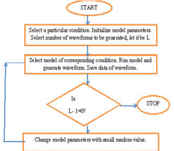
| The data for both networks is generated by the following algorithm, running the models described in the following sections. The algorithm for data generation for a particular condition is shown Fig 4. |
| IV.2.3 TRAINING |
| Using this data generated the network is trained so that ANN studies the features and characteristics of different signals. |
| For BPNN training input and target has to be given. Input is data generated in different conditions. Target is either 0 or 1. |
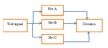
| For RBNN three networks are created ie. net A, net B and net C. Each network is created by combining one fault condition data and normal condition data. Net A is created by using data of internal fault without harmonics and normal condition. Net B is created by using data of internal fault with harmonics and normal condition. Similarly net C by combining external fault data and normal condition data. |
| For each network input and target values are given and trained. To each network we give fault condition data and normal data for setting the threshold for classifying the fault. Training architecture of Net A is shown in fig 6. |
| From training architecture each network is trained and fed with inputs from all the four models. The characteristic output for each network is determined for the particular fault condition. In other words, each network is tuned for producing a unique output when the fault corresponding to that fault condition for which it is trained. This information is used in the decision making block in the testing architecture |
| For classifying fault or testing the system. the test signal is generated from the model. The processed test signal can be either normal(no fault) or corresponding to a particular fault. This is passed to the neural network bank. The outputs from the neural network bank is compared and fault is classified accurately. |
| For BPNN first we select a particular condition for testing. Then we will send 8 test signals to the network generated. For each condition there is a threshold value. This threshold value will be a value between 0 and 1. Based on this threshold value fault classification is done. |
| For RBNN we will select a particular condition. Based on threshold value classification is done. Here threshold value will be 0 for fault condition and 1 for normal condition. |
| IV.2.4 RESULTS |
| In the case of BPNN first we will select normal condition. For normal condition threshold value is 0.37. Based on this threshold value fault classification is shown in Table 1. |
| Now for internal fault with harmonics, threshold chosen is 0.01. Fault classification is shown in Table 3. Next for internal fault without harmonics, threshold chosen is 0.52. Fault classification is shown in Table 4. |
| Now for RBNN if normal condition is selected the output of all networks is shown in Table 5. If internal fault without harmonics is selected output of each network is shown in Table 6. |
| From the above results we can see that when BPNN was used for fault classification in some cases there was incorrect results. This is because the threshold value selected was not accurate. When RBNN was used the outputs are either 0 or 1. For normal condition output of all network is high. The fault for a particular condition when fed to the network bank produces a low output for the network tuned for that particular condition and high for other conditions. Hence decision making become more robust and easy resulting in accurate fault classification. |
| The testing for faults resulted in nearly hundred percent accuracy in fault classification when RBNN was used. The accuracy of fault classification depends on the threshold value selected. By comparing both the neural networks the use of Radial basis network saves time as well as memory, and fast creation of network objects. Radial basis network is used where there is large amount of input data. |
V CONCLUSION
|
| A novel fault classification strategy for differential protection of transformers is presented. Fault classification is done by using Artificial Neural Network. Here both Back Propagation Neural Network and Radial Basis Neural Network is used. The fault signal is preprocessed and fed to the neural network bank tuned. The outputs shows that proposed fault classification technique result in accurate decision making when RBNN is used compared to BPNN. The use of Radial basis network saves time as well as memory, and fast creation of network objects. |
| |
Tables at a glance
|
 |
 |
 |
 |
| Table 1 |
Table 2 |
Table 3 |
Table 4 |
 |
 |
 |
 |
| Table 5 |
Table 6 |
Table 7 |
Table 8 |
|
Figures at a glance
|
 |
 |
 |
 |
| Figure 1 |
Figure 2 |
Figure 3 |
Figure 4 |
 |
 |
 |
 |
| Figure 5 |
Figure 6 |
Figure 7 |
Figure 8 |
|
| |
References
|
- Adel Aktaibi and M.Azizur Rahman, “ Digital Differential Protection of Power Transformer using MATLAB”
- J.A.Sykes, I.F.Morrison, “ A proposed method of harmonic restraint differential protection of transformer by digital computer” , IEEE TransPAS-91, p1266, 1972.
- R.R.Tarson, A.J.Flechsig, E.O.Schweitzer, “Design and test of a digital relay for transformer protection” , IEEE Trans PAS-98, p795, 1979 .
- O.P.Malik, P.K.Dash, G.S.Hope, “Digital Protection of power transformer” ,IEEE PES Winter meeting, New York, Paper A76 p-191, 1976 .
- R.Bouderbala, H.Bentarzi and A.Ouadi,“Digital differential relay reliability Enchancement of Power Transformer” International Journal ofCircuits,Systems and Signal Processing Issue 3,Vol 5,2011.
- Mohammed S Abdulrahem, Adel Ridha Othman, “Simulation of power transformer differential relay” Engg and Tech Journal, Vol 27, No16,2009.
- PrabhaKundur, “ Power System Stability and Control”, TataMcGraw-Hill edition, 1993.
- ManojTripathy, R.P.Maheshwari and H.K.Verma, “Improved transformer protection using probabilistic neural network and power differentialmethod” International Journal of Engineering.Vol.2,No.3,2010 .
- Thomas Dalstein, Bernd Kulickr, “Neural network apparoach to fault classification for high speed protective relaying” IEEE Trans on PowerDelivery, Vol 10, No 2, April 1995.
- 10.Thomas Dalstein, Thomas Friedrich, Bernd Kulickr, DejanSobajic, “Multi neural network based fault area estimation for high speed protectiverelaying”,IEEE Trans on Power Delivery, Vol 11, No 2, April 1996.
- Li Yongli, He Jiali, DuanYugian, “Application of neural network to microprocessor based transformer protective relaying”.
- 12.Uttamu Lahiri, A.K.Pradhan, S.Mukhopadhyaya, “Modular neural network based directional relay for transmission line protection” IEEEtranscations on power system, Vol 20,No:4, Nov 2005.
- 13.P.Chandra Sekhar, B.V.Sankar Ram, K.S.Sarma, “Fast computing neural network modeling for fault diagnosis in power system” APRNJournalogEngg and Applied science, Vol 5, No 9, Sept 2010.
- 14.Tripathy, R.P.Maheshwal and H.K.Verma”Radial basis probabilistic neural network for differential protection of power transformer” .
- ManojTripathy, “Power transformer protection using neural network principal component analysis and radial basis function neural network“ Simulation modeling practice and theory, Vol 18, Issue 5, May 2010.
- Chee-MunOng, “Dynamic simulation of Electric Machinary using Matlab/Simulink”.
- ABB Relays, “power transformer protection application guide” AGO-5005E, 1998
- Anderson P.M, “Power system protection” IEEE Pres, Mc-Graw Hill.
- M.C.Say, “Performance and design of AC machines”
- Alexander S Langsdorf, “Theory of alternating current machinery”
|