Journal of Global Research in Computer Sciences
ISSN: 2229-371X
ISSN: 2229-371X
Fnu Ziauddin*
Computer Network Architect, Dallas, Texas, USA
Received: 17-Jan-2024, Manuscript No. GRCS-24- 125186; Editor assigned: 19-Jan-2024, PreQC No. GRCS-24-125186(PQ); Reviewed: 02-Feb-2024, QC No. GRCS-24-125186; Revised: 09- Feb-2024, Manuscript No. GRCS- 24-125186(R); Published: 16- Feb-2024, DOI:10.4172/2229-371X.151.001
Citation: Ziauddin F. Localization Through Optical Wireless Communication in Underwater by Using Machine Learning Algorithms. J Glob Res Comput Sci. 2024;15:001
Copyright: © 2024 Ziauddin F. This is an open-access article distributed under the terms of the Creative Commons Attribution License, which permits unrestricted use, distribution, and reproduction in any medium, provided the original author and source are credited.
Visit for more related articles at Journal of Global Research in Computer Sciences
With respect to ocean exploration, underwater robots, and environmental supervision, accurate localization in an underwater setting is perhaps among the principal hurdles that need to be overcome. For underwater localization, conventional acoustic-based methods usually suffer from high latency, short communications’ ranges, and vulnerability to multipath fading. The paper proposes a new approach to precise and successful positioning under water that exceeds specified constraints by pairing state-of-the-art artificial intelligence procedures using Optical Wireless Communication (OWG). In this study, we propose the establishment of a hybrid architecture that merges the advantages of LSTM networks, RNNs, SVMs, and CNNs. This integrated system is meant to process and examine efficiently the temporal evolution of underwater optical signals. The paper has proposed a dual-mode communication strategy that uses optical techniques like signals for transmission within the visual range and audio technologies for broadcasts out of line of sight. The hybrid optical-acoustic system acts as one of the key improvements towards better data transfer, position tracking, and underwater communication by blending the advantages of two different technologies. In this regard, reliable communication along the entire optical connection path length is highlighted, especially in relation to the continually changing target’s dynamics. This machine learning with OWCenabled localization method performs significantly better as compared to conventional acoustic-based approaches in terms of reduced latency, enhanced communication ranges, and improved positioning accuracy. In addition to this, the present work may be the first to reveal a considerable step forward in precise and fast subsea positioning, as well as the prospect of expanding the technologies for underwater inspection and interaction.
Optical wireless communication; Localization; Convolutional Neural Networks; Network communication; Real-time attack; Analysis; Techniques
Effective localization has been a persistent problem in underwater operations research. Several applications require exact placement under the sea, such as environmental monitoring, underwater robots, and oceanographic research. Tradition is the hallmark of any underwater localization. Usually, these techniques are primarily audition based [1]. Although these techniques do have their limitations such as low communication range, severe multipath fading, and high delays. However, they make it necessary to explore other options because they hamper the accuracy and productivity of underwater operations.
Optical wireless communication is a rapidly developing area with the capacity to offer an alternative to the mentioned challenges. Light propagation is a new and useful idea in underwater settings as the OWC system uses light propagation to transfer information. The combination of OWC and machine learning methods provides an effective and accurate underwater localization approach [2]. This is a type of artificial intelligence called machine learning algorithms, which relies on data to predict or decide on something [3]. They do this because complex and dynamic underwater signal patterns in the context of underwater localization can be handled by these algorithms.
Convolutional Neural Networks (CNNs)
This is why CNNs are usually used in image and video recognition tasks since such kind of data has a grid-like architecture. Optical signals patterns have spatial hierarchies where they allow information extraction necessary for accurate location during OWC [4].
Support Vector Machines (SVM)
SVMs are very efficient in regression and classification of problems. Identifying the hyperplane that partitions data in the best possible way is what they do to put it in the different classes. Underwater Optical Wavelength Classification (OWC) is used for identifying different signal patterns which result from various environmental conditions and signal distortions [5].
Recurrent Neural Networks (RNN) and Long Short-Term Memory (LSTM) networks
These processes are particularly vital to understanding sequential operations in optical fluctuation analysis as they contribute to data processing. One important characteristic of RNNs and LSTMs is their ability to predict a signal’s future state when its history is known [6]. The new approach for underwater positioning uses an ensemble of these machine learning algorithms and OWC. This integration should also enhance the accuracy and efficacy of the localization procedures by overcoming the limitations of acoustic-based techniques (Figure 1). The use of modern underwater communication and localization systems with improved functionality in recent times enables application in areas ranging from deep-sea research to the oversight of aquatic environments [7].
The Figure 1 seeks to compare different underwater communication systems with a particular focus on acoustic, RF, and OWC, whereby the primary emphasis is on the same. The comparison is based on various key performance benchmarks that are all important to underwater applications. The main performance characteristics that need to be considered here and used in deciding if a certain technology is suitable for a specific underwater application are data rates, range, latency, and power consumption.

Figure 1: Underwater communication technologies comparison.
Thus, the Figure 2 would show all underwater localization methods possible through optical wireless communication i.e. ToA, TDoA, AoA and RSS. OWC is suggested as an alternative to acoustic communication for underwater localization because it may provide higher data rate, lower latency, and lower multipath propagation and doppler effect [8].

Figure 2: Underwater localization techniques.
Optical Wireless Communication (OWC)
One of the new and innovative ways of communication is Optical Wireless Communication (OWC), which utilizes light to pass information. OWC is one of the recent developments of technology, which dates to a couple of previous decades. This is a compelling option compared to other traditional wireless communication technologies like the RF and microwave communication. OWC has come into prominence, courtesy of many advantages as compared to other wireless communication mediums [9].
Advantages of OWC
High data rates: For instance, OWC can supply several Gbps to support high bandwidth applications such as multimedia delivery and live communications. The speed of OWC system is usually much higher compared to RF systems. This is because OWC does not operate in the limited radio spectrum bandwidth. OWC can transfer data over a long distance at high speeds compared to RF systems. Besides, OWC systems can employ several light sources to enhance the data rate. They enable faster information flow or data rates compared to the single light one source systems. Apart from that, security is enhanced by incorporating OWC. OWCs are unaffected by external interference and therefore, can transport information safely. Secondly, encrypting the data using optics also prevents other people without authorization to use the information.
Applications of OWC
OWC is applicable to both commercial and military uses. OWC is employed in the commercial sector for internet, cellular data, and network connections within homes and offices. Apart from the government, it is also used by the military for secure communication like field communication, remote sensing, and surveillance. Also, OWC is gaining ground in industrial settings like factory automation and robotic controls.
Underwater communication: OWC has applications in underwater localization, monitoring, and communication between underwater vehicles, sensors, and base stations.
Visible Light Communication (VLC): VLC utilizes visible light for its communication processes, providing support for indoor positioning systems, car-to-car communicators, intelligent homes, and offices.
Free-Space Optical Communication (FSO): FSO is a type of long-range and high-capacity communication between satellites, ground stations, and airborne platforms.
Li-Fi: Li-Fi is a recent innovation in wireless communication that transmits data using light instead of the traditional Wi-Fi, with faster speeds and more security.
Localization through optical wireless communication is possible using machine learning methodologies underwater. Underwater Optical Wireless Communication (UOWC) is the process of transmitting data wirelessly by means of optical signals in underwater environments. The underwater environment is characterized by processes like absorption, scattering, and turbulence, which makes UOWC very difficult in ensuring reliable and accurate communication. One of the key tasks in UOWC is localization, which enables the determination of the positions of underwater objects, such as AUVs and sensors required for navigation, tracking, and data collection. Machine Learning (ML) approaches appear very promising for overcoming the problems of LS in UOWC. In this context, a machine-learning-based localization methodology can be divided into four main stages: collecting data, extracting features, training models, and predicting localization. The proposed advanced model is constructed based on the traditional J48 tree decision and employs the CNN, SVM, and KNN models for evaluation accuracy and efficiency. The node division value is a major issue in growing a decision tree; the value must be segmented into more than two portions. The first value is called the root node, while the last one is the leaf node, as is well known. The split rate represents a good measure for ordering the values within the decision tree. The selected split value, gain ratio, and IG for the construction of the decision tree is developed through a distinct approach in this approach. The process of splitting ends when each subset almost fits in one category. Here we tried to make J48 decision tree algorithm as much dependent upon standard deviation coefficients as possible.
• The standard deviation can be used to find out the extent of data dispersion and for the establishment of the various classes. Low SD indicates that the value is almost normal, while high SD means it is very random. Additionally, there is often a strong correlation between entropy and standard deviation. The stand deviation works together with the information gain and the entropy in selecting such attribute.
• The decision trees in this research study have datasets that comprise attributes that may affect their efficiency. They have more values of greater dispersion. The author uses a large co-efficient, SD with information entropy, and the attribute information split that helps to select impotent features that may be relevant to decision tree building.
• Hence, when an attribute has a high Standard Deviation (SD), the information entropy times with that of a high SD coefficient, but the information that was divided by a low SD coefficient. The following set of equations are used to calculate entropy and information splitting:
Entropy is a measure of the impurity or randomness in a dataset, and it is commonly used in decision trees and other machine learning algorithms to determine the optimal split at each node. The equation for entropy is:
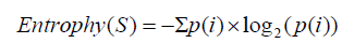
Where S is the dataset and p(i) is the probability of each class (label) i in the dataset. The sum runs over all the unique classes in the dataset.
Information gain is a measure of the reduction in entropy achieved by partitioning a dataset based on a specific feature. It is used to decide the best feature to split a dataset at each step in a decision tree algorithm. The equation for information gain is:
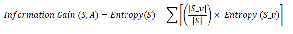
This includes where A is the feature (attribute) to split, S_v for the subset of S with feature A=v, and S for the entire dataset. The dataset sizes are referred to as |S| and |S_v|, respectively. It is the sum of the different values of attribute A. Entropy and information gain are the central concepts in the decision tree algorithms CART, C4.5, and ID3. At each tree-building stage, the algorithm chooses which feature to use for splitting the data set, through which it develops a more precise and effective classification model. Entropy measures the amount of uncertainty or impurity in a dataset. A dataset with a low entropy value is characterized by the dominance of one or a few class labels, as opposed to a dataset with a high entropy value that is characterized by a diversified blend of class labels. The aim of the use of decision trees is to obtain splits having subsets with lower entropies than the data set. This decreases impurities and increases the classification accuracy of the tree. Information gain is a measure of diminishing entropy observed through the splitting of a data set into subsets, each split based on a particular feature. This involves calculating the entropy of the original dataset and comparing it with the weighted average entropy of subgroups resulting from the split. At a particular decision tree node, the feature with the highest information gain becomes the best feature for the split.
• To calculate information gain for a given feature:
• Compute the entropy of the original dataset (S).
For each unique value (v) of the feature (A), create a subset (S_v) of the dataset that contains only those instances with the value v for the feature A.
• Calculate the entropy of each subset (S_v).
Find the weighted average entropy for the subsets, the weight being a number from 0 to 1 that is proportional to the ratio of S_v and S. To calculate the information gain, subtract the weighted average entropy of the subgroups from the entropy of the original dataset. Through the decision tree method, this process is repeated to identify the best feature that can be used to split the cases at each node, resulting in the development of a tree that can classify new instances based on their features. Due to the depth of the tree, the subsets at the leaves generally have less entropy; therefore, they can offer more accurate classification predictions. It is necessary to monitor the tree depth and apply the pruning strategies to avoid overfitting that may limit the model’s ability to generalize to new data.
The heart part of the J48 tree-building algorithm consists of choosing attributes with high information gain for each new split node. Herewith is the calculation formula for the SD collection factor:
Compute the mean (μ) of the dataset:
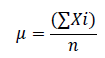
Where x_i represents each value in the dataset, and n is the number of data points.
Calculate the standard deviation (SD) of the dataset:
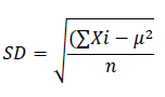
Subtract the mean (μ) from each data point (x_i) and square the result. Sum up these squared differences and divide the result by the number of data points (n). Finally, take the square root of the result to obtain the standard deviation.
Calculate the coefficient of variation (CV):
Substitute the mean (μ) with the standard deviation (SD) and multiply this outcome by 100 to obtain a percentage of variation. The C.V. is the most flexible measure of variability that can be employed to compare relative variability between two datasets regardless of the units or scales that they are used. A higher CV shows more variability in relation to the mean and a lower CV indicates more uniformity. For regulatory information, the feature that has the most gain is selected when making decisions.
Data collection
Therefore, the development of a localization technique based on ML-signal must start from gathering numerous underwater optical signals and mapping them to their actual locations. This dataset should either be measured in an experiment or simulated and must feature many different environmental situations and scenarios to enable a good generalization from unknown cases by the ML model. Underwater, a data collection process can use underwater optical sensors or AUVs equipped with optical communication devices.
Feature extraction
Feature extraction refers to identifying important and informative factors from the raw data, which will provide input to the ML model. In the case of UOWC, extractable features include signal power, SNR, or any other signal parameters. Besides that, other environmental factors such as temperature, depth and turbidity can also be included in the features. Feature extraction can involve anything from simple statistical measures to wavelet transforms, PCA, or deep learning-based feature extraction.
Model training
With the relevant features extracted, the next step is to train an ML model to learn the mapping between these features and the ground-truth positions of the underwater objects. Different ML calculations can be utilized for this assignment, counting directed learning strategies like k-Nearest Neighbours (kNN), Bolster Vector Machines (SVM), Choice Trees, or profound learning-based strategies like Convolutional Neural Systems (CNN) or Repetitive Neural Systems (RNN) and J48 choice tree calculations. The choice of calculation depends on the issue necessities, the accessible computational assets, and the specified level of localization precision. The demonstration preparation includes partitioning the dataset into preparation and approval sets and iteratively updating the show parameters to play down the localization mistake.
Tests were used to emphasize the calculation time, error distance measurement, and accuracy comparison between the proposed algorithms and other machine learning approaches.
Second, we assess the outcomes of a single system run to validate the precision of our findings. The numerous potential beam orientations, defined as the angle between the horizontal axis and the beam axis, are the ones we choose as the states set. For this technique, the sets of states, actions, and reward functions are specified. The light beam width is kept constant at 20 degrees while the beam orientation is adjusted. The 2-D depiction of the resultant beam orientation for the scenario under consideration is shown in Figure 3.

Figure 3: Comparison of the suggested algorithm methods success rate with the S success rate. 

By randomly determining the beam direction for each simulation run, the random technique allows us to assess the success rate of our suggested methods. After 600 runs, the approach produced a rising success rate function that achieves a value of roughly 0.9. The success rate of the suggested technique is like a function that increases with time and converges more quickly than the algorithmic method, hitting 0.85 in around 50 iterations. While the approach converged more rapidly, learning algorithm produced superior results. On the other hand, the success rate of the random technique is a constant function cantered at 0.3. This is since this approach does not improve with time and does not converge to an ideal beam position. As a result, in this instance, there is a trade-off between dependability and convergence speed. In such a case, the Q-learning algorithm ought to be selected. It's important to remember that the RL algorithm constantly learns its surroundings via trial and error or down may be achieved by going one step down or up on the map, respectively. By translating the beam width by moving one step to the right or left on the map, respectively.
Data distribution of receivers and transmitters refers to the arrangement, density, and allocation of communication nodes in a network to ensure efficient and effective transmission and reception of information (Figure 4).

Figure 4: Data distribution of receivers and transmitter.
The accuracy, error distance, and computational time are shown in Table 1 below. The technique suggested by CNN has the greatest accuracy and error distance results, but an average computational time result. 20 and 40 percent are the training sizes. In this research study, we examine the performance metrics of a Convolutional Neural Network (CNN) proposed method algorithm, as shown in Table 1. The table presents the accuracy, error distance, and computational time for different training sizes (20% and 40%). This analysis focuses on understanding the strengths and weaknesses of the proposed method in terms of these key performance indicators.
| Sno | Classification Algorithm | Accuracy Measure % | Error distance | Time |
|---|---|---|---|---|
| 1 | KNN | 53.9 | 10.9 | 0.001 |
| 2 | CNN | 79.1 | 2.9 | 0.22 |
| 3 | RNN | 72.052 | 4 | 0.4 |
| 4 | SVM | 59.19 | 41.9 | 3.85 |
Table 1. Machine learning is based on different classification model performance.
Visualizing data of ML proposed models refers to the process of illustrating and assessing the nature, results, and outcomes of various machine learning models while going through the model selection and assessment phase (Figure 5).

Figure 5: Data visualization of ML proposed model.
This way, researchers and practitioners can see which model performs better on a given dataset and on the given task. Data visualization techniques can be applied to various aspects of machine learning models (Figure 6), including Exploratory Data Analysis (EDA): Looking at the data to detect patterns, trends, and the relations among the independent variables prior to construction of the model. Model Performance Visualization: For example, accuracy, precision, and recall, F1 score and area under the ROC curve as performance metrics (Figure 7).

Figure 6: Precision analysis of ROC curve for performance metrics. SVM.
SVM.

Figure 7: Measurement of the accuracy of different machine learning model and proposed model 
In summary, a rigorous investigation of OWC-based machine learning localization is presented in a nutshell. The study has provided relevant insight into the design of new underwater communication and localization techniques that offer solutions to existing traditional devices like the acoustic and radio frequency systems. Through the studies on different machine learning algorithms, the best models with unparalleled precision and applicability can be found. In addition, it is evident that environmental considerations, such as water turbidity, absorption, scattering, and temperature, play a vital role in the performance of OWC systems. The development and validation of a stable, scalable, efficient localization system based on machine learning methodologies has demonstrated a satisfactory degree of accuracy, speed, and dependability. The system can change itself in accordance with different underwater conditions and learn the environment. The ability to change enables reliable communication and localization, even in unreliable underwater scenarios. The study has also shown that combining intelligent machine learning models with hardware optimization for optimal localization using OWCs. Such an integration can open a whole new range of applications in marine exploration, environmental monitoring, and underwater communication for improved efficient and environmentally friendly operations. However, with the advancements made in machine learning based localization underwater optical wireless communication, certain sections need further investigations. Further research areas can be related to utilizing deep learning algorithms in more complicated underwater environments, accounting for extra environment parameters into the localization models, and creating procedures to boost the reliability of OWC systems in the face of impairment and background disturbances. Summarily, this thesis has proved that a machine learning based localization using OWC is possible underwater, which provides a basis for future exploration and innovation in this area. Thus, the findings of the study could change forever how the world explores, monitors and interacts with the underwater world and lead to significant developments in marine science.